BE 150/Bi 250b Lecture 5: Analysis of Feed Forward Loops
(c) 2018 Justin Bois. With the exception of pasted graphics, where the source is noted, this work is licensed under a Creative Commons Attribution License CC-BY 4.0. All code contained herein is licensed under an MIT license.
This document was prepared at Caltech with support financial support from the Donna and Benjamin M. Rosen Bioengineering Center.

This tutorial was generated from a Jupyter notebook. You can download the notebook here.
# NumPy and odeint, our workhorses
import numpy as np
import scipy.integrate
# Plotting modules
import bokeh.io
import bokeh.plotting
# Bokeh color palette
colors = bokeh.palettes.d3['Category10'][10]
# Ensure that plots show in the notebook
bokeh.io.output_notebook()
In this lecture, we will discuss the feed forward loop, or FFL. We discovered in the previous lecture that this is a prevalent motif in E. coli. That is to say that the FFL appears more often, in fact much more often, in circuits present in E. coli that would be expected by random chance. As Prof. Elowitz said in the last lecture, given the prevalence of FFLs, they most likely are doing something. To get to the bottom of this, we will do a full analysis of them in this lecture.
Categorizing FFLs
The architecture of the FFL was discussed in the last lecture. It consists of three genes, which we will call X, Y, and Z. We think of X as an input that regulates both Y and Z. Y regulates Z. The regulation can be either activating or repressing (or something more complicated, but we will restrict our attention to these two). So, there are three interactions to consider, X's regulation of Y, X's regulation of Z, and Y's regulation of Z. There are two choices of mode of regulation for each, so there are a total of $2^3 = 8$ different FFLs. These are shown below, in a figure taken from Alon, Nature Rev. Genet., 8, 450--461, 2007. Abbreviations for these circuits are commonly used. E.g., C2-FFL is the coherent FFL of type 2 and I4-FFL is the incoherent FFL of type 4.
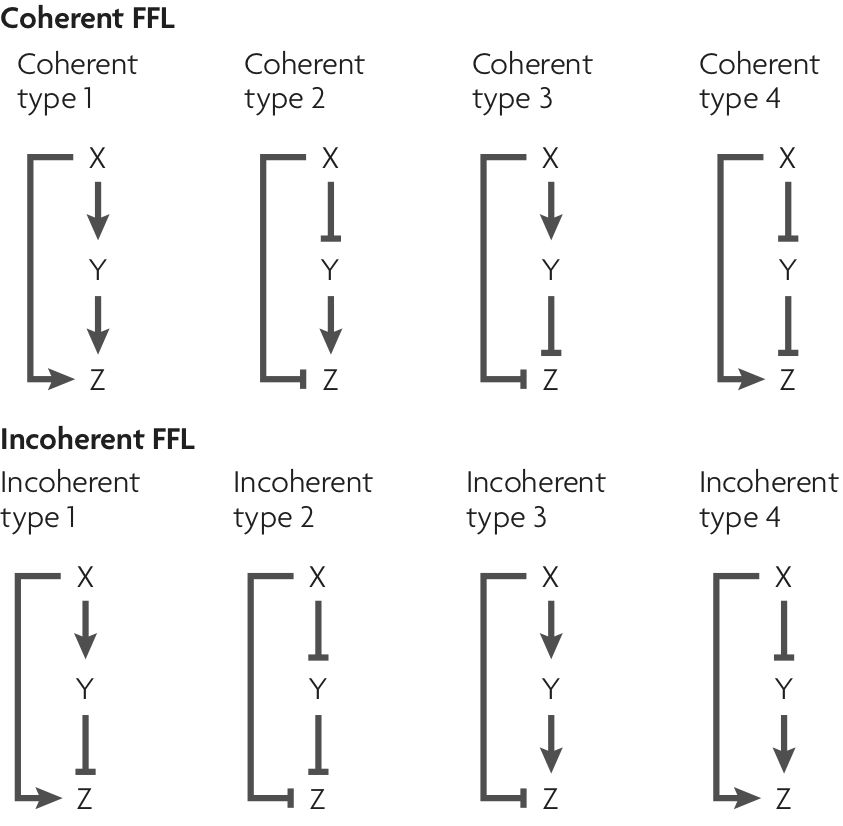
Half of the FFL architectures are coherent and half are incoherent. For those that are coherent, X's direct regulation of Z and its indirect regulation of Z are the same, either both activating or both repressing. For incoherent FFLs, X's direct and indirect regulation are not the same.
The most-encountered FFLs
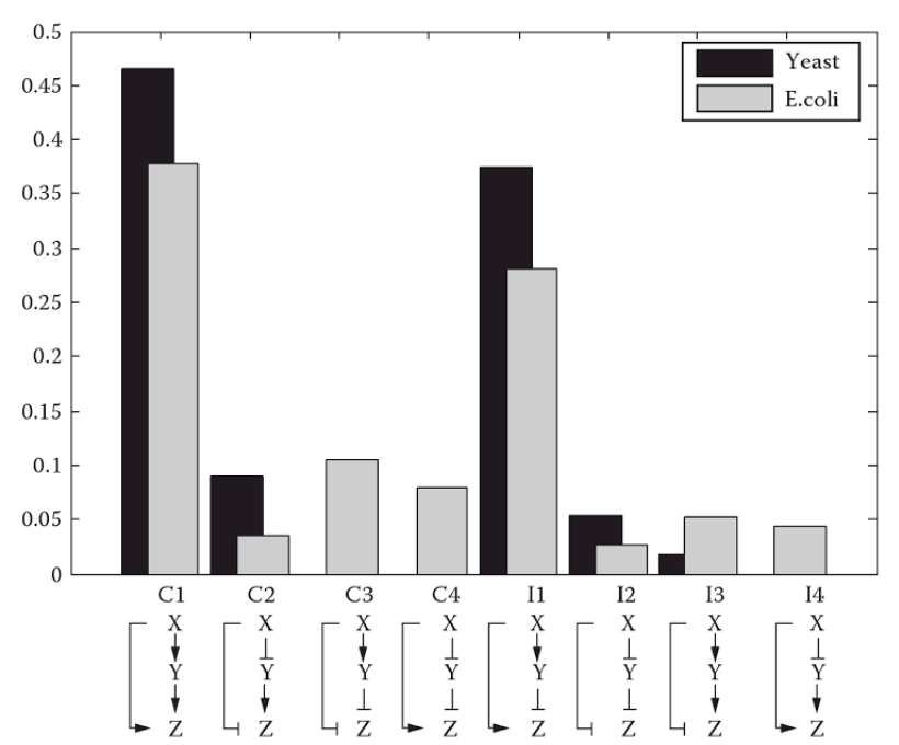
While FFLs in general are motifs, some FFLS are more often encountered than others. In the figure below, also taken from the Alon review, we see relative abundance of the eight different FFLs in E. coli and S. cerevisiae. Two FFLs, C1-FFL and I1-FFL stand out as having much higher abundance than the other six. Let's take a look at these two FFLs in turn to see what features they might provide.
Logic of regulation by two transcription factors
Because X and Y both regulate Z in an FFL, we need to specify how they do that.
For the sake of illustration, let us assume we are discussing C1-FFL, where X activates Z and Y also activates Z. One can imagine a scenario where both X and Y need to be present to turn on Z. For example, they could be binding partners that together serve to recruit polymerase to the promoter. We call this AND logic. In other words, to get expression of Z, we must have X AND Y. Conversely, if either X or Y may alone activate Z, we have OR logic. That is, to get expression of Z, we must have X OR Y.
So, to fully specify an FFL, we need to also specify the logic of how Z is regulated. So, we might have, for example, a C1-FFL with OR logic. This gives a total of 16 possible FFLs.
We are now left with the task of figuring out how to encode AND and OR logic.
Logic with two activators
Let us start first with Y and Z both activating with AND logic. We can construct a truth table for whether or not Z is on, given the on/off status of X and Y. The truth table is shown below, with a zero entry meaning that the gene is not on and a one entry meaning it is on.
| X | Y | Z |
|---|---|---|
| 0 | 0 | 0 |
| 0 | 1 | 0 |
| 1 | 0 | 0 |
| 1 | 1 | 1 |
We can also construct a truth table for OR logic with X and Y both activating.
| X | Y | Z |
|---|---|---|
| 0 | 0 | 0 |
| 0 | 1 | 1 |
| 1 | 0 | 1 |
| 1 | 1 | 1 |
As a reminder, the dynamics of the concentration of Z may be written as
\begin{align} \frac{\mathrm{d}z}{\mathrm{d}t} = \beta_0\,f(x, y) - \gamma z. \end{align}
Our goal is to specify the dimensionless function $f(x, y)$. How do we encode it with Hill functions? We could derive the functional form from the molecular details of the promoter region and the activators. Instead, we will again use a phenomenological Hill function. (Again, we could show that these Hill functions match certain promoter architectures.) The following functions work.
\begin{align} &\text{AND logic: } f(x,y) = \frac{(x/k_x)^{n_x} (y/k_y)^{n_y}}{1 + (x/k_x)^{n_x} (y/k_y)^{n_y}},\\[1em] &\text{OR logic: } f(x,y) = \frac{(x/k_x)^{n_x} + (y/k_y)^{n_y}}{1 + (x/k_x)^{n_x} + (y/k_y)^{n_y}}. \end{align}
In what follows, we will take $x/k_x \to x$ and $y/k_y \to y$ such that $x$ and $y$ are not dimensionless, nondimensionalized by their Hill $k$. In this notation, we have
\begin{align} &\text{AND logic: } f(x,y) = \frac{x^{n_x} y^{n_y}}{1 + x^{n_x} y^{n_y}},\\[1em] &\text{OR logic: } f(x,y) = \frac{x^{n_x} + y^{n_y}}{1 + x^{n_x} + y^{n_y}}. \end{align}
We can make plots of these functions to demonstrate how they resprensent the respective logic.
def contourf(x, y, z, title=None):
"""Make a filled contour plot given x, y, z data given in 2D arrays."""
p = bokeh.plotting.figure(plot_height=300,
plot_width=325,
x_range=(x.min(), x.max()),
y_range=(y.min(), y.max()),
x_axis_label='x',
y_axis_label='y',
title=title)
p.image(image=[z],
x=x.min(),
y=y.min(),
dw=x.max()-x.min(),
dh=x.max()-x.min(),
palette='Viridis11')
return p
# Get x and y values for plotting
x = np.linspace(0, 2, 500)
y = np.linspace(0, 2, 500)
xx, yy = np.meshgrid(x, y)
# Parameters (steep Hill functions)
nx = 20
ny = 20
# Regulation functions
def aa_and(x, y, nx, ny):
return x**nx * y**ny / (1 + x**nx * y**ny)
def aa_or(x, y, nx, ny):
return (x**nx + y**ny) / (1 + x**nx + y**ny)
# Generate plots
plots = [contourf(xx, yy, aa_and(xx, yy, nx, ny), title='two activators, AND logic'),
contourf(xx, yy, aa_or(xx, yy, nx, ny), title='two activators, OR logic')]
bokeh.io.show(bokeh.layouts.row(plots))
With AND logic, both X and Y must have high concentrations for Z to be expressed. Conversely, for OR logic, either X or Y can be in high concentrations for Z to be expressed, but if neither is high enough, Z does not get expressed. The equations phenomenologically capture the logic.
Logic with two repressors
Now let's consider the case where we have two repressors, as in the C3-FFL or I2-FFL. The AND case where X and Y are both repressors is NOT X AND NOT Y. This is equivalent to a NAND gate, with the following truth table.
| X | Y | Z |
|---|---|---|
| 0 | 0 | 1 |
| 0 | 1 | 1 |
| 1 | 0 | 1 |
| 1 | 1 | 0 |
We might get this kind of logic if the two repressors need to work in concert, perhaps through binding interactions, to affect repression.
For OR logic with two repressors, we have have NOT X OR NOT Y, which is a NOR gate. Its truth table is below.
| X | Y | Z |
|---|---|---|
| 0 | 0 | 1 |
| 0 | 1 | 0 |
| 1 | 0 | 0 |
| 1 | 1 | 0 |
Here, either repressor (or both) can shut down gene expression. We can encode these with dimensionless regulation functions
\begin{align} &\text{AND logic: } f(x,y) = \frac{1}{(1 + x^{n_x}) (1 + y^{n_y})},\\[1em] &\text{OR logic: } f(x,y) = \frac{1 + x^{n_x} + y^{n_y}}{(1 + x^{n_x}) ( 1 + y^{n_y})}. \end{align}
Let's make some plots to see how these functions look.
# Regulation functions
def rr_and(x, y, nx, ny):
return 1 / (1 + x**nx) / (1 + y**ny)
def rr_or(x, y, nx, ny):
return (1 + x**nx + y**ny) / (1 + x**nx) / (1 + y**ny)
# Generate plots
plots = [contourf(xx, yy, rr_and(xx, yy, nx, ny), title='two repressors, AND logic'),
contourf(xx, yy, rr_or(xx, yy, nx, ny), title='two repressors, OR logic')]
bokeh.io.show(bokeh.layouts.row(plots))
Logic with one activator and one repressor
Now say we have one activator (which we will designate to be X) and one repressor (which we will designate to be Y). Now, AND logic means X AND NOT Y, and OR logic means X OR NOT Y. The truth table for the AND gate is below.
| X | Y | Z |
|---|---|---|
| 0 | 0 | 0 |
| 0 | 1 | 0 |
| 1 | 0 | 1 |
| 1 | 1 | 0 |
And that for the OR gate is
| X | Y | Z |
|---|---|---|
| 0 | 0 | 1 |
| 0 | 1 | 0 |
| 1 | 0 | 1 |
| 1 | 1 | 1 |
The dimensionless regulatory functions are
\begin{align} &\text{AND logic: } f(x,y) = \frac{x^{n_x}}{(1 + x^{n_x} + y^{n_y})},\\[1em] &\text{OR logic: } f(x,y) = \frac{1 + x^{n_x}}{(1 + x^{n_x} + y^{n_y})}. \end{align}
Finally, let's look at a plot.
# Regulation functions
def ar_and(x, y, nx, ny):
return x**nx / (1 + x**nx + y**ny)
def ar_or(x, y, nx, ny):
return (1 + x**nx) / (1 + x**nx + y**ny)
# Generate plots
plots = [contourf(xx, yy, ar_and(xx, yy, nx, ny), title='X activates, Y represses, AND logic'),
contourf(xx, yy, ar_or(xx, yy, nx, ny), title='X activates, Y represses, OR logic')]
bokeh.io.show(bokeh.layouts.row(plots))
The CFFL-1 circuit enables sign-sensitive delay
We will now proceed to an analysis of the first of the two over-represented FFLs, the C1-FFL. We will take X as an input and then write down dynamical equations for the concentrations of Y and Z. We will start with AND logic.
\begin{align} \frac{\mathrm{d}y}{\mathrm{d}t} &= \beta_y\,\frac{(x/k_{xy})^{n_{xy}}}{1 + (x/k_{xy})^{n_{xy}}} - \gamma_y y, \\[1em] \frac{\mathrm{d}z}{\mathrm{d}t} &= \beta_z\,\frac{(x/k_{xz})^{n_{xz}} (y/k_{yz})^{n_{yz}}}{1 + (x/k_{xz})^{n_{xz}} (y/k_{yz})^{n_{yz}}} - \gamma_z z, \end{align}
where we have used the notation that $k_{ij}$ is the Hill k for j regulated by i, with $n_{ij}$ similarly defined. To nondimensionalize these equations, we will take
\begin{align} t &= \tilde{t} / \gamma_y, \\[1em] x &= k_{xz}\,\tilde{x},\\[1em] y &= k_{yz}\,\tilde{y},\\[1em] z &=z_0\,\tilde{z}, \end{align}
where $z_0$ is as of yet unspecified. Substituting these expressions in and rearranging, we have, dropping tildes for notational convenience,
\begin{align} \frac{\mathrm{d}y}{\mathrm{d}t} &= \frac{\beta_y}{\gamma_y k_{yz}}\,\frac{(\kappa x)^{n_{xy}}}{1 + (\kappa x)^{n_{xy}}} - y, \\[1em] \gamma^{-1}\frac{\mathrm{d}z}{\mathrm{d}t} &= \frac{\beta_z}{z_0\gamma_z}\,\frac{x^{n_{xz}} y^{n_{yz}}}{1 + x^{n_{xz}} y^{n_{yz}}} - z. \end{align}
Here, we have defined $\kappa \equiv k_{xz}/k_{xy}$ and $\gamma \equiv \gamma_z/\gamma_y$. We are free to choose $z_0$ to be what we like, and $z_0 = \beta_z/\gamma_z$ is a convenient choice. Finally, we redefine $\beta_y$ to get the dimensionless version $\beta_y \leftarrow \beta_y/\gamma_y k_{yz}$. We when have our dimensionless dynamical system.
\begin{align} \frac{\mathrm{d}y}{\mathrm{d}t} &= \beta_y\,\frac{(\kappa x)^{n_{xy}}}{1 + (\kappa x)^{n_{xy}}} - y, \\[1em] \gamma^{-1}\frac{\mathrm{d}z}{\mathrm{d}t} &= \frac{x^{n_{xz}} y^{n_{yz}}}{1 + x^{n_{xz}} y^{n_{yz}}} - z. \end{align}
Now that we have the dynamical equations, we can solve it numerically. For ease, when we define the right hand side of the dynamical system, we will also include OR logic.
Ideally, we would build a Bokeh app to explore the dynamics of the circuit for various parameter values, but for the pedagogical purposes of exposing design principles here, we will vary the parameters one-by-one.
To start, we code up some useful functions for the stimulus, the right hand side of the system of ODEs for the C1-FFL, and plotting utility.
def x_pulse(t, t_0, tau, x_0):
"""
Returns x value for a pulse beginning at t = 0
and ending at t = t_0 + tau.
"""
return np.logical_and(t >= t_0, t <= (t_0 + tau)) * x_0
def c1ffl(yz, t, beta_y, kappa, gamma, n_xy, n_xz, n_yz, logic, x_fun, x_args):
"""Right hand side of dynamics of C1-FFL"""
# Unpack
y, z = yz
# Evaluate x
x = x_fun(t, *x_args)
# y-derivative
dy_dt = beta_y * (kappa*x)**n_xy / (1 + (kappa*x)**n_xy) - y
# x-derivative
if logic == 'and':
dz_dt = gamma * (aa_and(x, y, n_xz, n_yz) - z)
elif logic == 'or':
dz_dt = gamma * (aa_or(x, y, n_xz, n_yz) - z)
return np.array([dy_dt, dz_dt])
def plot_dynamics(t, yz, x_fun, x_args, normalized=False, normalize_to_max=True):
"""Convenient plotting function for results"""
p = bokeh.plotting.figure(plot_height=200,
plot_width=600,
x_axis_label='dimensionless time',
y_axis_label='dimensionless conc.')
# Get plot of stimulus dynamics
if t[-1] > x_args[0] + x_args[1]:
t_x = np.array([0, x_args[0], x_args[0], x_args[0]+x_args[1], x_args[0]+x_args[1], t[-1]])
x = np.array([0, 0, x_args[2], x_args[2], 0, 0])
else:
t_x = np.array([0, x_args[0], x_args[0], t[-1]])
x = np.array([0, 0, x_args[2], x_args[2]])
if normalized:
if normalize_to_max:
p.line(t_x, x/x.max(), line_width=2, color=colors[0], legend='x')
p.line(t, yz[:,0]/yz[:,0].max(), line_width=2, color=colors[1], legend='y')
p.line(t, yz[:,1]/yz[:,1].max(), line_width=2, color=colors[2], legend='z')
else:
p.line(t_x, x/x[-1], line_width=2, color=colors[0], legend='x')
p.line(t, yz[:,0]/yz[-1,0], line_width=2, color=colors[1], legend='y')
p.line(t, yz[:,1]/yz[-1,1], line_width=2, color=colors[2], legend='z')
else:
p.line(t_x, x, line_width=2, color=colors[0], legend='x')
p.line(t, yz[:,0], line_width=2, color=colors[1], legend='y')
p.line(t, yz[:,1], line_width=2, color=colors[2], legend='z')
return p
With these convenient functions available, we can now specify parameters, solve, and plot.
# Parameter values
beta_y = 5
kappa = 1
gamma = 1
n_xy, n_yz = 3, 3
n_xz = 5
logic = 'and'
t_0 = 1
tau = 10
x_0 = 1
t = np.linspace(0, 15, 200)
# Initial condition
yz0 = np.array([0, 0])
# Set up and solve
x_args = (t_0, tau, x_0)
args = (beta_y, kappa, gamma, n_xy, n_xz, n_yz, logic, x_pulse, x_args)
yz = scipy.integrate.odeint(c1ffl, yz0, t, args)
# Plot
bokeh.io.show(plot_dynamics(t, yz, x_pulse, x_args))
Notice that there is a time delay for production of Z upon stimulation with X. However, there is no delay when the signal X is turned off. The z curve responds immediately. This is perhaps more apparent if we normalize the signals.
bokeh.io.show(plot_dynamics(t, yz, x_pulse, x_args, normalized=True))
Here, the delay is more apparent, as is the fact that both Y and Z have their levels immediately decrease when the X stimulus is removed.
So, we have arrived at a design principle, The C1-FFL with AND logic has an on-delay, but no off-delay.
The magnitude of the delay can be tuned with κ
How might we get a longer delay? If we decrease $\kappa = k_{xz}/k_{yz}$, we are increasing the disparity between the threshold levels needed to turn on gene expression. This should result in a longer time delay. Let's try it!
# Update parameter
kappa = 0.1
# Set up args and solve
args = (beta_y, kappa, gamma, n_xy, n_xz, n_yz, logic, x_pulse, x_args)
yz = scipy.integrate.odeint(c1ffl, yz0, t, args)
# Plot
bokeh.io.show(plot_dynamics(t, yz, x_pulse, x_args, normalized=True))
Indeed, the delay is longer with small κ.
The delay does not require ultrasensitivity
We might think that ultrasensitivity is required for the delay, but it is not.
# No ultrasensitivity
n_xy, n_xz, n_yz = 1, 1, 1
# Set up args and solve
args = (beta_y, kappa, gamma, n_xy, n_xz, n_yz, logic, x_pulse, x_args)
yz = scipy.integrate.odeint(c1ffl, yz0, t, args)
# Plot
bokeh.io.show(plot_dynamics(t, yz, x_pulse, x_args))
Without ultrasensitivity, the delay is shorter, but present nonetheless. This is because with AND logic, the expression of Z still has to wait for Y to get high enough to begin producing Z at an appreciable level.
The C1-FFL with AND logic and filter out short pulses
Now, let's see what happens if we have a shorter pulse. Due to its similarly with the cascade we studied last week, the delay feature of the C1-FFl should also filter our short pulses.
# Shorter pulse
t_0 = 0.1
tau = 0.2
t = np.linspace(0, 2, 200)
# Reset kappa and ultrasensitivity
kappa = 1
n_xy, n_xz, n_yz = 3, 5, 3
# Set up and solve
x_args = (t_0, tau, x_0)
args = (beta_y, kappa, gamma, n_xy, n_xz, n_yz, logic, x_pulse, x_args)
yz = scipy.integrate.odeint(c1ffl, yz0, t, args)
# Plot
bokeh.io.show(plot_dynamics(t, yz, x_pulse, x_args))
The shorter pulse is ignored because of the delay.
The sign-sensitivity of the delay is reversed with OR logic
We will now investigate the response of the circuit to the same stimulus, except with OR logic.
# Reset stimulus parameters
t_0 = 1
tau = 10
t = np.linspace(0, 15, 200)
# Use OR logic
logic = 'or'
# Set up and solve
x_args = (t_0, tau, x_0)
args = (beta_y, kappa, gamma, n_xy, n_xz, n_yz, logic, x_pulse, x_args)
yz = scipy.integrate.odeint(c1ffl, yz0, t, args)
# Plot
bokeh.io.show(plot_dynamics(t, yz, x_pulse, x_args))
Now we see that both Y and Z immediately start being produced upon stimulus, but there is a delay in the decrease of Z when the stimulus is removed. As with the AND logic, this is perhaps more easily seen with normalized concentrations.
# Plot
bokeh.io.show(plot_dynamics(t, yz, x_pulse, x_args, normalized=True))
The level of Z in a C1-FFL with OR logic does respond to a pulse in X, but, analogously to the case with AND logic, it ignores a quick decrease and increase in X.
The I1-FFL with AND logic is a pulse generator
We now turn our attention to the other over-represented circuit, the I1-FFL. As a reminder, here is the structure of the circuit.
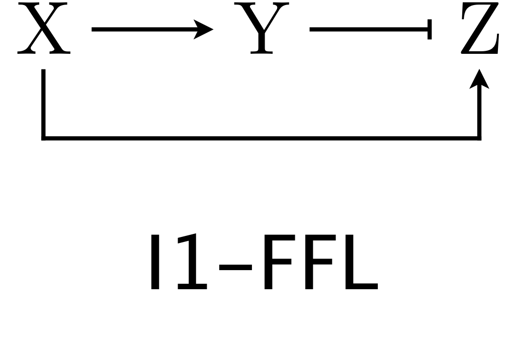
X activates Y and Z, but Y represses Z. We can use the expressions for production rate under AND and OR logic for one activator/one repressor that we showed above in writing down our dynamical equations. Here, we will consider AND logic. Nondimensionalization proceeds as in the C1-FFL example. The dimensionless dynamical equations are
\begin{align} \frac{\mathrm{d}y}{\mathrm{d}t} &= \beta_y\,\frac{(\kappa x)^{n_{xy}}}{1+(\kappa x)^{n_{xy}}} - y,\\[1em] \gamma^{-1}\,\frac{\mathrm{d}z}{\mathrm{d}t} &= \frac{x^{n_{xz}}}{(1 + x^{n_{xz}} + y^{n_{yz}})} - z. \end{align}
We can code this up.
def i1ffl(yz, t, beta_y, kappa, gamma, n_xy, n_xz, n_yz, logic, x_fun, x_args):
"""Right hand side of dynamics of C1-FFL"""
# Unpack
y, z = yz
# Evaluate x
x = x_fun(t, *x_args)
# y-derivative
dy_dt = beta_y * (kappa*x)**n_xy / (1 + (kappa*x)**n_xy) - y
# x-derivative
if logic == 'and':
dz_dt = gamma * (ar_and(x, y, n_xz, n_yz) - z)
elif logic == 'or':
dz_dt = gamma * (ar_or(x, y, n_xz, n_yz) - z)
return np.array([dy_dt, dz_dt])
Now, let's use it to observe the dynamics of an I1-FFL. We will investigate the response in Z to a sudden, sustained step in stimulus X.
# Parameter values
beta_y = 3
kappa = 1
gamma = 10
n_xy, n_yz = 3, 3
n_xz = 5
logic = 'and'
t_0 = 1
tau = 10
x_0 = 1
t = np.linspace(0, 10, 200)
# Initial condition
yz0 = np.array([0, 0])
# Set up and solve
x_args = (t_0, tau, x_0)
args = (beta_y, kappa, gamma, n_xy, n_xz, n_yz, logic, x_pulse, x_args)
yz = scipy.integrate.odeint(i1ffl, yz0, t, args)
# Plot
bokeh.io.show(plot_dynamics(t, yz, x_pulse, x_args))
We see that Z pulses up and then falls down to its steady state value. This is because the presence X leads to production of Z due to its activation. X also leads to the increase in Y, and once enough Y is present, it can start to repress Z. This brings the Z level back down toward a new steady state where the production rate of Z is a balance between activation by X and repression by Y. Thus, the I1-FFL with AND logic is a pulse generator.
The I1-FFL with AND logic gives an accelerated response
Let us compare the response of an I1-FFL being suddenly turned on (by a step in X) to an unregulated circuit that achieves the same steady state. Recall that the dimensionless dynamics for the unregulated circuit follow
\begin{align} z(t) = 1 - \mathrm{e}^{-t}. \end{align}
If we plot the normalized I1-FFL together with the unregulated response, we see that the I1-FFl makes it to the steady state faster, though it overshoots and then relaxes.
p = bokeh.plotting.figure(plot_height=200,
plot_width=600,
x_axis_label='dimensionless time',
y_axis_label='dimensionless conc.')
# I1-FFL dynamics
inds = t > t_0
t = t[inds] - t_0
p.line(t, yz[:,1][inds]/yz[-1,1], line_width=2, color=colors[2], legend='I1-FFL')
# Unregulated dynamics
p.line(t, 1 - np.exp(-t), line_width=2, color=colors[4], legend='unregulated')
bokeh.io.show(p)
So, we have another design principle, The I1-FFL with AND logic has a faster response time than an unregulated circuit.