Stochastic differentiation

(c) 2018 Justin Bois. With the exception of pasted graphics, where the source is noted, this work is licensed under a Creative Commons Attribution License CC-BY 4.0. All code contained herein is licensed under an MIT license.

This document was prepared at Caltech with financial support from the Donna and Benjamin M. Rosen Bioengineering Center.

This tutorial was generated from an Jupyter notebook. You can download the notebook here.

As usual, we will import the modules we'll use first.

# Workhorses
import numpy as np
import scipy.integrate

# Plotting modules
import matplotlib.pyplot as plt
import seaborn as sns
sns.set(style='whitegrid', context='notebook')

# This is to enable inline displays for the purposes of the tutorial
%matplotlib inline
%config InlineBackend.figure_formats = {'png', 'retina'}

# Interactive plotting
import bokeh.plotting
import bokeh.io
import ipywidgets
bokeh.io.output_notebook()

BokehJS 0.12.15 successfully loaded.

Dynamical equations

The reduced representation of the competence circuit is shown below (taken from Süel, et al., Nature, 2006).

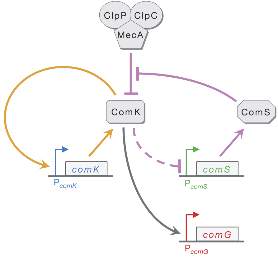
The ClpP/ClpC/MecA complex degrades ComK and ComS. For brevity, we will just call the complex "MecA." ComS serves to inhibit this degradation by tying up the MecA complex in degrading itself. That is, there are two competing reactions: degradation of ComK and degradation of ComS. We take both of these reaction to have Michaelis-Menten kinetics, giving the reaction schemes

$$\begin{align} &\text{MecA} + \text{ComK} \stackrel{\gamma_{\pm a}}{\rightleftharpoons} \text{MecA-ComK} \stackrel{\gamma_1}{\rightarrow} \text{MecA} \\[1em] &\text{MecA} + \text{ComS} \stackrel{\gamma_{\pm b}}{\rightleftharpoons} \text{MecA-ComS} \stackrel{\gamma_2}{\rightarrow} \text{MecA}. \end{align}$$

ComK is also known to indirectly inhibit expression of ComS, denoted by the dashed arrow. We take this to be described by a Hill function. Finally, ComK has a basal expression level. We can therefore write the dynamical equations for ComK and the MecA-ComK complex as

$$\begin{align} \frac{\mathrm{d}K}{\mathrm{d}t}&= \alpha_k + \beta_k\,\frac{K^n}{k_k^n + K^n} - \gamma_a M_f K + \gamma_{-a}M_K,\\[1em] \frac{\mathrm{d}M_K}{\mathrm{d}t} &= -(\gamma_{-a} + \gamma_1)M_K + \gamma_aM_f K, \end{align}$$

where we have denoted the concentration of MecA-ComK as $M_K$ and of free MecA as $M_f$. We has assumed that degradation by the MecA complex overwhelms the natural degradation of the protein product.

We write the influence of ComK on ComS expression as a repressive Hill function. With our assumption of Michaelis-Menten kinetics on ComS degradation by MecA, we can now write the dynamical equations for ComS and the ComS-MecA complex.

$$\begin{align} \frac{\mathrm{d}S}{\mathrm{d}t}&= \frac{\beta_s}{1 + (K/k_s)^p} - \gamma_b M_f S + \gamma_{-b}M_S,\\[1em] \frac{\mathrm{d}M_S}{\mathrm{d}t} &= -(\gamma_{-b} + \gamma_2)M_S + \gamma_b M_f S. \end{align}$$

Now, if we assume that the conversion of the MecA-Com complexes are very fast ($\gamma_1$ and $\gamma_2$ are large), we can make a pseudo-steady state approximation such that $\mathrm{d}M_K/\mathrm{d}t \approx \mathrm{d}M_S/\mathrm{d}t \approx 0$. Finally, if we assume that the total amount of MecA complex is conserved, i.e., $M_f + M_K + M_S = M_\mathrm{total} \approx \text{constant}$, we can simply our expressions. Specifically, we now have

$$\begin{align} \frac{\mathrm{d}K}{\mathrm{d}t}&= \alpha_k + \beta_k\,\frac{K^n}{k_k^n + K^n} -\gamma_1M_K,\\[1em] \frac{\mathrm{d}S}{\mathrm{d}t}&= \frac{\beta_s}{1 + (K/k_s)^p} - \gamma_2 M_S. \end{align}$$

We can get expressions for $M_K$ and $M_S$ in terms of $M_\mathrm{total}$, $K$, and $S$ by using the relations

$$\begin{align} -(\gamma_{-a} + \gamma_1)M_K + \gamma_a(M_\mathrm{total} - M_K - M_S) K &= 0\\[1em] -(\gamma_{-b} + \gamma_2)M_S + \gamma_b(M_\mathrm{total} - M_K - M_S) S &= 0. \end{align}$$

We can write these in a more convenient form to eliminate $M_K$ and $M_S$.

$$\begin{align} (\gamma_{-a} + \gamma_1 + \gamma_a K)M_K + \gamma_a K M_S &= \gamma_a M_\mathrm{total} K \\[1em] \gamma_b S M_K + (\gamma_{-b} + \gamma_2 + \gamma_b S)M_S &= \gamma_b M_\mathrm{total} S. \end{align}$$

Solving this system of linear equations for $M_K$ and $M_S$ yields

$$\begin{align} M_K &= M_\mathrm{total}\,\frac{K/\Gamma_k}{1 + K/\Gamma_k + S/\Gamma_s}, \\[1em] M_S &= M_\mathrm{total}\,\frac{S/\Gamma_s}{1 + K/\Gamma_k + S/\Gamma_s}, \end{align}$$

where $\Gamma_k \equiv (\gamma_{-a} + \gamma_1)/\gamma_a$ and $\Gamma_k \equiv (\gamma_{-b} + \gamma_2)/\gamma_b$. Inserting these expressions back into our ODEs for the $K$ and $S$ dynamics yields

$$\begin{align} \frac{\mathrm{d}K}{\mathrm{d}t}&= \alpha_k + \beta_k\,\frac{K^n}{k_k^n + K^n} -\gamma_1 M_\mathrm{total}\,\frac{K/\Gamma_k}{1 + K/\Gamma_k + S/\Gamma_s} \\[1em] \frac{\mathrm{d}S}{\mathrm{d}t}&= \frac{\beta_s}{1 + (K/k_s)^p} - \gamma_2 M_\mathrm{total}\,\frac{S/\Gamma_s}{1 + K/\Gamma_k + S/\Gamma_s}. \end{align}$$

For simplicity in modeling our system, we will take $\gamma_1 \approx \gamma_2$.

With this in place, we can nondimensionalize the two dynamical equations. We take $s = S/\Gamma_s$ and $k = K/\Gamma_k$. We take dimensionless time to be $\gamma_1 M_\mathrm{total} t$. As a result, we get dimensionless equations

$$\begin{align} \frac{\mathrm{d}k}{\mathrm{d}t}&= a_k + b_k\,\frac{k^n}{\kappa_k^n + k^n} - \frac{k}{1 + k + s} - \gamma_k k, \\[1em] \frac{\mathrm{d}s}{\mathrm{d}t}&= a_s + \frac{b_s}{1 + (k/\kappa_s)^p} - \frac{s}{1 + k + s} - \gamma_s s. \\ &\phantom{nada} \end{align}$$

Analysis of the dynamical system

Now that we have our dynamic system set up, we can begin analysis. We will start by defining parameters for the system. We will use the parameters specified in the Süel, et al. papers.

class CompetenceParams(object):
    """
    Container for parameters for B. subtilis competence circuit.
    """
    def __init__(self, paper_year=2007, **kwargs):
        # Dimensionless parameters
        if paper_year == 2007:
            self.a_k = 0.00035
            self.a_s = 0.0
            self.b_k = 0.3
            self.b_s = 3.0
            self.kappa_k = 0.2
            self.kappa_s = 1/30
            self.gamma_k = 0.1
            self.gamma_s = 0.1
            self.n = 2
            self.p = 5
        elif paper_year == 2006:
            self.a_k = 0.004
            self.b_k = 0.07
            self.b_s = 0.82
            self.kappa_k = 0.2
            self.kappa_s = 0.222
            self.gamma_k = 0
            self.gamma_s = 0
            self.n = 2
            self.p = 5
        else:
            raise RuntimeError('Invalid paper year.')
        
        # Put in params that were specified in input
        for entry in kwargs:
            setattr(self, entry, kwargs[entry])    

It is also useful to define the time derivatives.

def dk_dt(k, s, p):
    return p.a_k + p.b_k * k**p.n / (p.kappa_k**p.n + k**p.n) \
                    - k / (1 + k + s) - p.gamma_k*k

def ds_dt(k, s, p):
    return p.a_s + p.b_s / (1 + (k / p.kappa_s)**p.p) - s / (1 + k + s) - p.gamma_s*s

We can also define functions for the nullclines. These are curves that are $s(k)$, that is, $s$ as a function of $k$. These are easily derived by setting $\mathrm{d}k/\mathrm{d}t$ and $\mathrm{d}s/\mathrm{d}t$ equal to zero.

def dk_dt_nullcline(k, p):
    abk = p.a_k + p.b_k * k**p.n / (p.kappa_k**p.n + k**p.n) - p.gamma_k * k
    return k / abk - k - 1

def ds_dt_nullcline(k, p):
    bk = p.a_s + p.b_s / (1 + (k / p.kappa_s)**p.p)
    a = p.gamma_s
    b = 1 - bk + p.gamma_s * (1 + k)
    c = -bk * (1 + k)

    return -2*c / (b + np.sqrt(b**2 - 4*a*c))

We can also write a generic function for plotting flow fields in the phase portrait. This is a useful function to have around in general.

def plot_flow_field(ax, du_dt, dv_dt, u_range, v_range, p, log=False):
    """
    Plots the flow field with line thickness proportional to speed.
    """
    if log:
        # Set up u,v space
        log_u = np.linspace(np.log10(u_range[0]), np.log10(u_range[1]), 100)
        log_v = np.linspace(np.log10(v_range[0]), np.log10(v_range[1]), 100)
        log_uu, log_vv = np.meshgrid(log_u, log_v)

        # Compute derivatives
        log_u_vel = du_dt(10**log_uu, 10**log_vv, p) / 10**log_uu
        log_v_vel = dv_dt(10**log_uu, 10**log_vv, p) / 10**log_vv

        # Compute speed
        speed = np.sqrt(log_u_vel**2 + log_v_vel**2)

        # Make linewidths proportional to speed, with minimal line width of 0.5
        # and max of 5
        lw = 0.5 + 4.5 * speed / speed.max()

        # Make stream plot
        ax.streamplot(log_uu, log_vv, log_u_vel, log_v_vel, linewidth=lw, arrowsize=1.5, 
                       density=1.25, color=sns.color_palette()[0])
    else:
        # Set up u,v space
        u = np.linspace(u_range[0], u_range[1], 100)
        v = np.linspace(v_range[0], v_range[1], 100)
        uu, vv = np.meshgrid(u, v)

        # Compute derivatives
        u_vel = du_dt(uu, vv, p)
        v_vel = dv_dt(uu, vv, p)

        # Compute speed
        speed = np.sqrt(u_vel**2 + v_vel**2)

        # Make linewidths proportional to speed, with minimal line width of 0.5
        # and max of 5
        lw = 0.5 + 4.5 * speed / speed.max()

        # Make stream plot
        ax.streamplot(uu, vv, u_vel, v_vel, linewidth=lw, arrowsize=1.5, 
                       density=1.25, color=sns.color_palette()[0])

    return ax

We'll write a convenient function to compute and plot the nullclines as well.

def plot_nullclines(ax, k_range, log=False):
    """
    Compute and plot the nullclines.
    """
    if log:
        k = np.logspace(np.log10(k_range[0]), np.log10(k_range[1]), 200)
        s_nck = dk_dt_nullcline(k, p)
        s_ncs = ds_dt_nullcline(k, p)
        ax.plot(np.log10(k), np.log10(s_nck), '-', color=sns.color_palette()[3], lw=4)
        ax.plot(np.log10(k), np.log10(s_ncs), '-', color=sns.color_palette()[4], lw=4)
    else:
        k = np.linspace(k_range[0], k_range[1], 200)
        s_nck = dk_dt_nullcline(k, p)
        s_ncs = ds_dt_nullcline(k, p)
        ax.plot(k, s_nck, '-', color=sns.color_palette()[3], lw=4)
        ax.plot(k, s_ncs, '-', color=sns.color_palette()[4], lw=4)

    return ax

Now that we have all of this in place, we can compute and plot the flow field with the nullclines.

# Set paramters
p = CompetenceParams(2007)
k_range = [1e-3, 2]
s_range = [1e-2, 1000]

# Build figure
fig, ax = plt.subplots()
ax = plot_flow_field(ax, dk_dt, ds_dt, k_range, s_range, p, log=True)
ax = plot_nullclines(ax, k_range, log=True)

# Tidy up
ax.set_xlim(np.log10(k_range))
ax.set_ylim(np.log10(s_range))
ax.set_xlabel('$\log_{10}(k)$')
ax.set_ylabel('$\log_{10}(s)$');

We see that there are three fixed points. Let's zoom in on each fixed point and investigate them one by one. We'll start with the fixed point with smallest $k$.

k_range = [0.0025, 0.0030]
s_range = [10, 30]

# Build figure
fig, ax = plt.subplots()
ax = plot_flow_field(ax, dk_dt, ds_dt, k_range, s_range, p)
ax = plot_nullclines(ax, k_range)

# Tidy up
ax.set_xlim(k_range)
ax.set_ylim(s_range)
ax.set_xlabel('$k$')
ax.set_ylabel('$s$');

We see that this is a stable fixed point, with the system flowing into it. Let's now look at the fixed point for the next largest $k$.

k_range = [0.014, 0.02]
s_range = [10, 30]

# Build figure
fig, ax = plt.subplots()
ax = plot_flow_field(ax, dk_dt, ds_dt, k_range, s_range, p)
ax = plot_nullclines(ax, k_range)

# Tidy up
ax.set_xlim(k_range)
ax.set_ylim(s_range)
ax.set_xlabel('$k$')
ax.set_ylabel('$s$');

We can see from the flow lines that this is an unstable fixed point, a saddle. We could perform linear stability analysis on this fixed point, and we would find a positive trace and a negative determinant of the linear stability matrix.

Finally, let's look at the last fixed point, for largest $k$.

k_range = [0.02, 0.05]
s_range = [1, 10]

# Build figure
fig, ax = plt.subplots()
ax = plot_flow_field(ax, dk_dt, ds_dt, k_range, s_range, p)
ax = plot_nullclines(ax, k_range)

# Tidy up
ax.set_xlim(k_range)
ax.set_ylim(s_range)
ax.set_xlabel('$k$')
ax.set_ylabel('$s$');

This fixed point is a spiral source. It is unstable and spirals the system away from it.

Numerical solution of dynamical equations

We can numerically solve the dynamical equations. Of course, the initial conditions are relevant here. We will start with no ComK or ComS (which is not at all relevant physiologically) and solve.

# Right-hand-side of ODEs
def rhs(ks, t, p):
    """
    Right-hand side of dynamical system.
    """
    k, s = ks
    return np.array([dk_dt(k, s, p), ds_dt(k, s, p)])

# Set up and solve
t = np.linspace(0, 200, 100)
ks_0 = np.array([0, 0])
ks = scipy.integrate.odeint(rhs, ks_0, t, args=(p,))
k, s = ks.transpose()

# Plot result
fig, ax = plt.subplots(1, 2, figsize=(12, 4))
ax[0].plot(t, k/k.max())
ax[0].plot(t, s/s.max())
ax[0].set_xlabel('$t$')
ax[0].set_ylabel('normalized conc.')
ax[0].legend(('$k$', '$s$'), loc='lower right')
ax[0].margins(0.02)

ax[1].plot(k, s)
ax[1].set_xlabel('$k$')
ax[1].set_ylabel('$s$')
ax[1].margins(0.02)

We see a rise to the fixed point. This is not quite as interesting as watching this thing evolve on the phase diagram. We'll make an interactive graphic to do this.

pl = bokeh.plotting.figure(width=600, height=400, x_axis_label='k', 
                           y_axis_label='s', x_range=[0.001, 3], y_range=[1e-1, 1e3],
                           x_axis_type='log', y_axis_type='log')

# Plot nullclines
k_plot = np.logspace(-3, 1.5, 200)
s_nck = dk_dt_nullcline(k_plot, p)
s_ncs = ds_dt_nullcline(k_plot, p)
pl.line(k_plot, s_nck, color='#816FB3', line_width=4)
pl.line(k_plot, s_ncs, color='#C2B26F', line_width=4)

# Plot trajectory
pl.line(k, s, line_width=2, color='gray')
line = pl.line([k[0]], [s[0]], line_width=2)
dot = pl.circle([k[0]], [s[0]], size=10)

handle1 = bokeh.io.show(pl, notebook_handle=True);

def update(time=0.0):
    i = np.searchsorted(t, time)
    dot.data_source.data['x'] = [k[i]]
    dot.data_source.data['y'] = [s[i]]
    bokeh.io.push_notebook(handle=handle1)
    
time_slider = ipywidgets.FloatSlider(min=t[0], max=t[-1], value=t[0])

ipywidgets.interact(update, time=time_slider);

Now, let's say we had some fluctuation that kicked us up a bit in our ComS and ComK concentrations. We'll start with $s = 6$ and $k = 0.05$.

# Set up and solve
t = np.linspace(0, 200, 300)
ks_0 = np.array([1e-2, 1e3])
ks = scipy.integrate.odeint(rhs, ks_0, t, args=(p,))
k2, s2 = ks.transpose()

pl2 = bokeh.plotting.figure(width=600, height=400, x_axis_label='k', 
                           y_axis_label='s', x_range=[0.001, 2], y_range=[1e-3, 1e3],
                           x_axis_type='log', y_axis_type='log')

# Plot nullclines
k_plot = np.logspace(-3, np.log10(2), 200)
s_nck = dk_dt_nullcline(k_plot, p)
s_ncs = ds_dt_nullcline(k_plot, p)
pl2.line(k_plot, s_nck, color='#816FB3', line_width=4)
pl2.line(k_plot, s_ncs, color='#C2B26F', line_width=4)

# Plot trajectory
pl2.line(k2, s2, line_width=2, color='gray')
line = pl2.line([k2[0]], [s2[0]], line_width=2)
dot2 = pl2.circle([k2[0]], [s2[0]], size=10)

time_slider = ipywidgets.FloatSlider(min=t[0], max=t[-1], value=t[0])

handle2 = bokeh.io.show(pl2, notebook_handle=True);

def update2(time=0.0):
    i = np.searchsorted(t, time)
    dot2.data_source.data['x'] = [k2[i]]
    dot2.data_source.data['y'] = [s2[i]]
    bokeh.io.push_notebook(handle=handle2)

ipywidgets.interact(update2, time=time_slider);

This looks interesting. We made an excursion out to high $k$ before coming back.

This excursion is transient, which is important. We can get transient competence, returning back to the vegetative fixed point. To trigger an excursion, we simply need a small kick from the vegetative fixed point, which could be accomplished by noise.