1. Introduction to Biological Circuit Design
(c) 2019 Justin Bois and Michael Elowitz, except for images taken from sources where cited. This work is licensed under a Creative Commons Attribution License CC-BY 4.0. All code contained herein is licensed under an MIT license.
This document was prepared at Caltech with financial support from the Donna and Benjamin M. Rosen Bioengineering Center.

This lesson was generated from a Jupyter notebook. Click the links below for other versions of this lesson.
Key concepts for this lecture
- Genetic circuits control diverse biological behaviors
- The goals of the course are twofold:
- Understand the principles that explain the organization of natural biological circuits (systems biology) and allow the design of novel synthetic circuits that implement new cellular behaviors (synthetic biology).
- Develop tools and techniques for analyzing different circuit designs analytically and computationally.
- To facilitate the second goal, we will distribute lecture notes as executable Jupyter notebooks (like this one).
- "Design principles" provide functional rationales for choosing one circuit design or architecture over another, and are usually of the form Feature X provides function Y.
- Ordinary differential equations for protein production and removal allow analysis of simple gene expression processes.
- Separation of time scales allows us to ignore "faster" reactions when analyzing "slower" processes.
- Gene regulation can be analyzed in terms of binding of activators and repressors to binding sites.
Course Information
- The course will be TA'd by Andy Halleran and Tyler Ross
- Texts:
- Uri Alon, An Introduction to Systems Biology (note: 2nd edition will be released July 5, 2019)
- Steven Strogatz, Nonlinear Dynamics and Chaos
- Many lectures will follow corresponding chapters in Alon
- Professors: Justin Bois, Michael Elowitz
- Course website with lecture schedule, contact information, policies, etc.
- Piazza-hosted discussion group (linked from course website)
- Topics are subject to change
- Devices: Laptops & phones are black holes that suck human energy out of the room. Please refrain. Notes and/or slides will be distributed after each lecture to facilitate active participation. Paper notes are fine.
Biological circuit design
Living cells and the multicellular organisms they comprise represent (arguably) the most amazing systems in the universe! Each cell is, in some sense, just a membrane-bound collection of molecules. However, these molecules, interacting with one another, somehow manage to obtain and utilize nutrients, avoid toxins, control their own replication, enable the cell to grow and divide, keep track of time, coordinate with other cells to build multicellular tissues, organs, and organisms, and continue to evolve even more impressive functions. Without complaining.
In this course, we will study biological circuits from a design point of view. With that first sentence, we must immediately define what we mean by a biological circuit, and what we mean by design.
What is a biological circuit?
For this course, we will think about at least two levels of biological circuitry:
Molecular circuits operating in cells consist of molecular species (genes, proteins, etc.) that interact in specific ways with one another. For example, a gene can be transcribed to produce a specific mRNA, which can in turn be translated to produce a specific protein species. Similarly, a kinase may specifically phosphorylate a protein substrate on a specific residue. Specificity in these interactions is the key property that allows these interactions to act like circuits. The key variables in these circuits are the concentrations and sometimes the locations of different molecular species.
Examples of molecular circuits include those that control the cell cycle and the circadian clock, the signaling pathways that process signals from other cells, and the circuits that control cell death, among countless others.
One level up, we will also consider cell circuits. In this case, we can think of cells in different states (or different cell types) that signal to one another to control one another's growth, death, proliferation, and differentiation. The key variables in these circuits are the concentrations and locations of cells in different states.
Examples of cell circuits include the immune system, in which different cell types influence each other's proliferation and differentiation through cytokines and other signals.
Of course, the two levels are not independent. The behavior of a given cell type within a cell circuit is controlled by its molecular circuits.
Biological circuits provoke fundamental questions
The biological science have amassed a tremendous amount of information about the molecular components of cells (genes, RNAs, proteins, metabolites, and many other molecules) and their interactions. We can now say where transcription factors bind genome-wide, which proteins chemically modify which others, and which proteins function together in complexes. So from an analytical point of view, it seems (somewhat naively) as if we ought to be able to predict and control cellular behaviors with great precision. At the same time, synthetic biology approaches now allow us to construct new genetic circuits within cells that can program totally new behaviors.
These capabilities provoke some basic question about biological circuit design:
- What capabilities does each circuit or pathway provide for the cell? (function, design principles)
- How do these capabilities emerge from pathway architecture? (mechanism)
- How can we control cells in predictable ways using these pathways? (biomedical applications)
- How can we use circuit design principles to program new developmental behaviors in living cells? (synthetic biology and bioengineering)
- How can or should synthetic circuits be similar or different from natural circuits?
In this course, we will approach these questions from the point of view of both natural and synthetic circuits, with the idea that the fundamental principles that allow a circuit to function effectively within or among cells do not necessarily depend on whether that circuit evolved naturally or was constructed in the lab. Having said that, we also recognize that evolution may be able to produce designs that are more complex or different from those we are currently able to construct, or even conceive. In fact, a major goal of the course is to see to what extent we can learn principles from natural circuits that will allow us to design synthetic circuits more effectively.
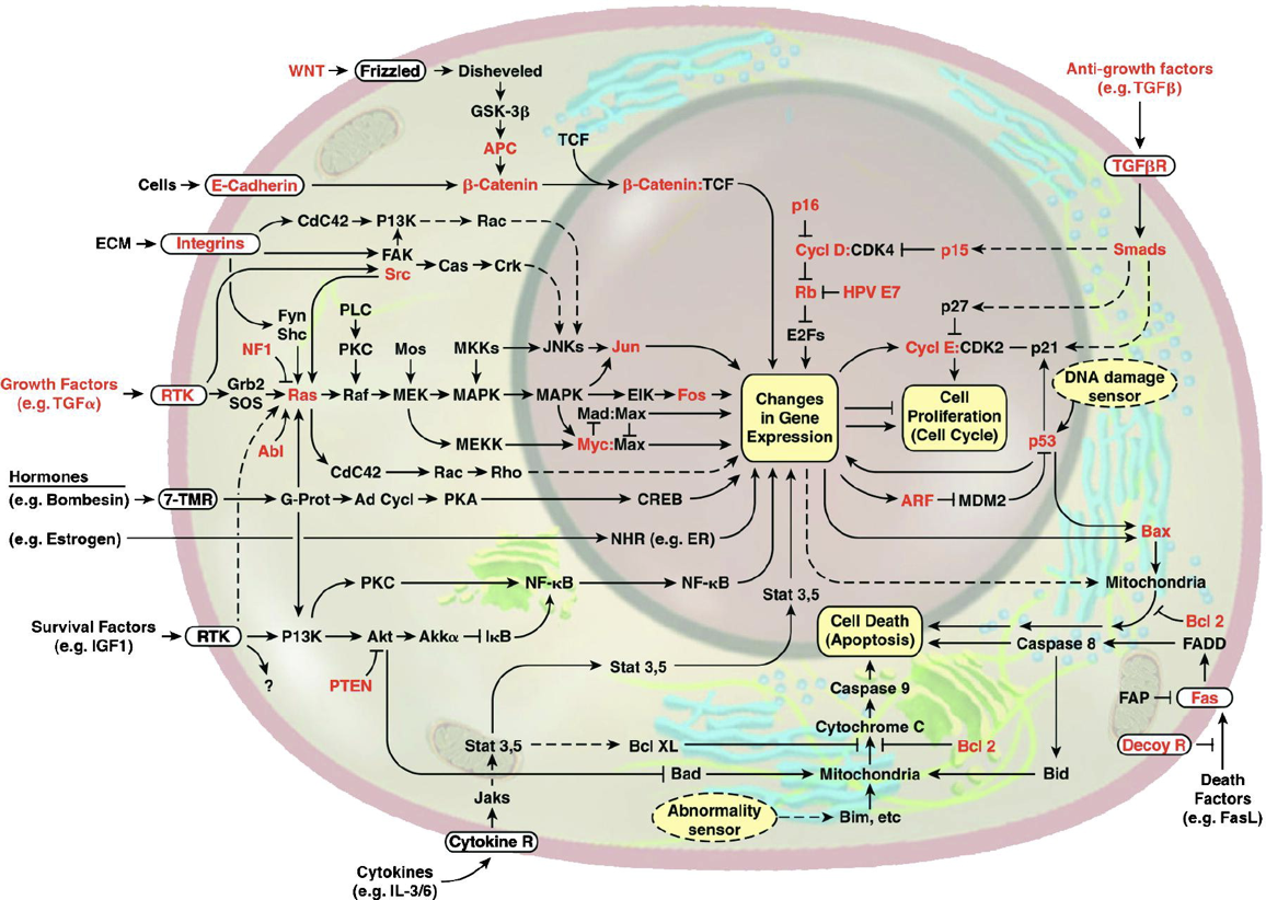
This image of the cell as a set of circuits comes from a classic review of cancer by Hanahan and Weinberg, Cell, 200081683-9).
Biological circuits differ from many other types of circuits or circuit-like systems
Electronic circuits, software, plumbing, construction, and many other human designed systems are based on connections between simple modular components (see Figure). We have well established design principles for many of these systems. Can we just apply those principles directly to living cells?
- Natural circuits were not designed by people! They evolved. That means they are not "well documented" and their function(s) are often totally unclear.
- Even synthetic circuits, which are designed by people, often use evolved components (such as transcription factors) for which we do not have a complete understanding.
- Unlike electronic circuits, which use wires to eliminate undesired crosstalk among components, biological circuits seem to exhibit extensive many-to-many interactions among their components.
- While electronic circuits can function deterministically, biological circuits exhibit function with high levels of stochastic (random) fluctuations in their own components. These fluctuations are often called "noise." And noise is not just a nuisance: some biological circuits take advantage of it to enable behaviors that would not be possible without it.
- Biological circuits can be highly parallel, in the sense that the same circuit can operate in many different genetically identical individual cells, whether in a bacterial population or in a multicellular organism, such as yourself.
- Electrical systems use positive or negative voltages and currents, allowing for positive or negative effects. By contrast, biological circuits are built out of molecules (or cells) whose concentrations cannot be negative. That means they must use other mechanisms for "inverting" activities.
- From a more practical point of view, we have a very limited ability to construct, test, and compare designs. Even with recent developments such as CRISPR, our ability to rapidly and precisely produce cells with well defined genomes remains limited compared to what is possible in more advanced disciplines. (Having said that, the situation is rapidly improving!)
- What others can you think of?
Inspiration from electronics
We can get some inspiration for thinking about biological circuit design from electronics. In their classic book, The Art of Electronics, Horowitz and Hill explain something similar to the excitement many now feel now about biology:
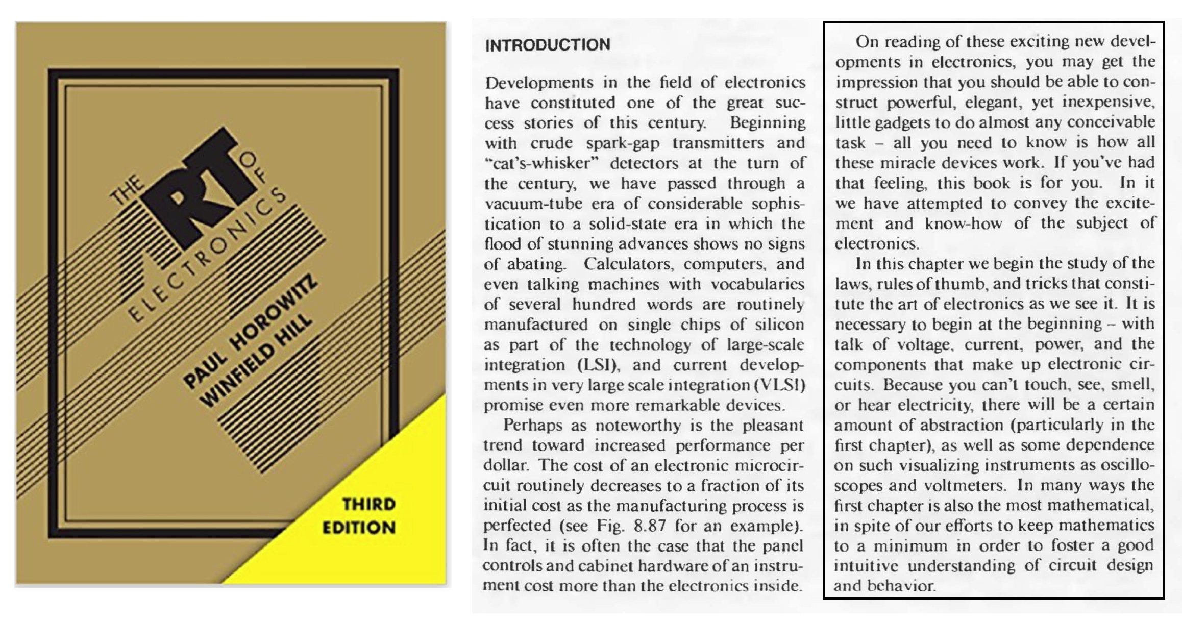
Paul Horowitz and Winfield Hill, The Art of Electronics, 3rd edition, Cambridge University Press, 2015.
Premise and goals of the course
Here we start from the premise that determining the design principles of genetic circuits will enable us to
- Understand, predict, and control living systems (systems biology)
- Design new genetic circuits that function effectively in cells and organisms (synthetic biology).
We also believe that our ability to formulate and use these design principles requires:
- A set of quantitative methods and approaches for analyzing different circuits
- New concepts and principles that can provide insight into rationale for different circuit designs
Therefore, the key goals for this course are to:
- Understand a broad spectrum of genetic circuit design principles from molecules to cells to tissues
- Develop quantitative methods to analyze and design genetic circuits
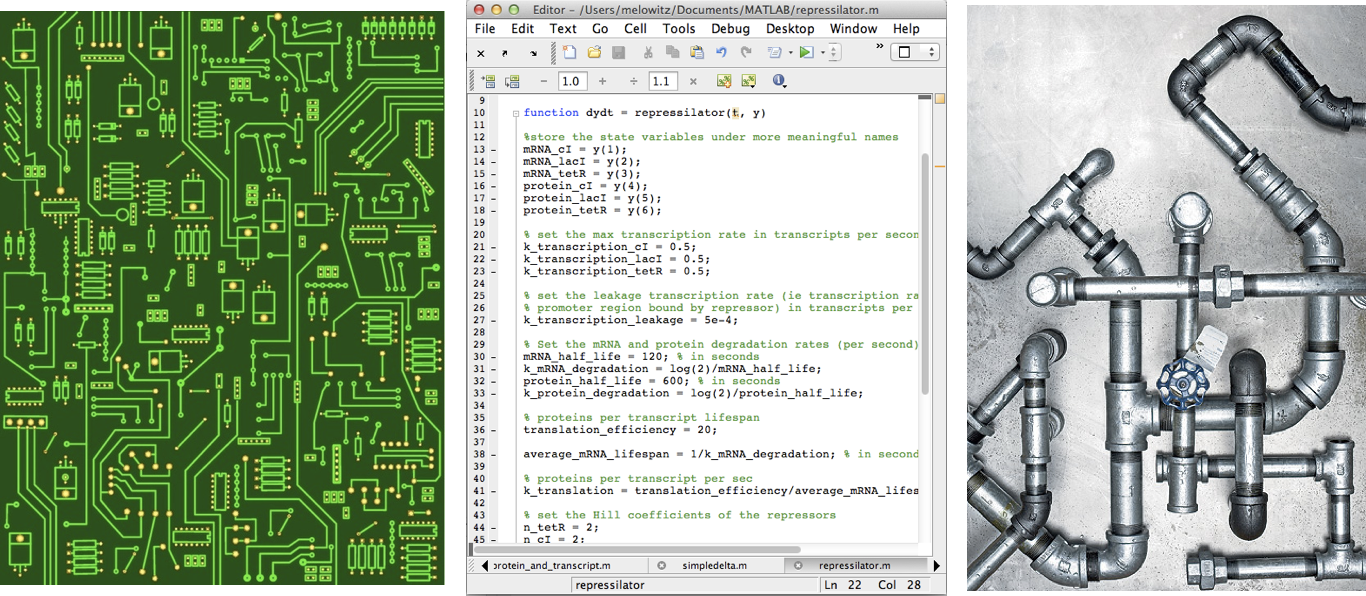
Electronics, software, and plumbing are great examples of human-designed systems that possess many properties analogous to biological circuits. These systems are based on known designed principles that sometimes overlap with, and sometimes differ from, those of biological circuits.
What is a gene circuit design principle?
We will define a circuit design principle as a statement of the form: Circuit feature X enables function Y. Each module of the course will explore a different design principle. Here are some examples:
- Negative autoregulation of a transcription factor accelerates its response to a change in input.
- Kinases that also act as phosphatases (bifunctional kinases) provide tunable linear amplifiers in two-component signaling systems.
- Pulsing a transcription factor on and off at different frequencies (time-based regulation) can enable coordinated regulation of many target genes.
- Noise-excitable circuits enable cells to control the probability of transiently differentiating into an alternate state
- Mutual inactivation of receptors and ligands in the same cell enable equivalent cells to signal unidirectionally
- Independent tuning of gene expression burst size and frequency enables cells to control cell-cell heterogeneity in gene expression
- Feedback on morphogen mobility allows tissue patterns to scale with the size of a tissue
- And many others...
Step one: Develop intuition for the simplest gene regulation circuits
We will start by thinking about a single gene, coding for a protein. Our goals are two-fold: First, develop intuition for the simplest possible gene expression system. Second, to lay out a procedure that we can extend to analyze more complex circuits.
What controls the level of the protein produced by gene x? We assume that the gene will be transcribed to mRNA and those mRNA molecules will in turn be translated to produce proteins, such that new proteins are produced at a total rate $\beta$ molecules per unit time. The protein does not simply accumulate over time. It is also removed both through active degradation as well as dilution as cells grow and divide. For simplicity, we will assume that both processes tend to reduce protein concentrations through a simple first-order process, with a rate constant $\gamma$.
(The approach we are taking can be described as "phenomenological modeling." We are not modeling every underlying molecular step. Instead, we are assuming that the underlying molecular steps give rise to 'coarse grain' relationships that we can model in a manner that is independent of the underlying details. The test of this approach is the extent to which it allows us to understand and experimentally predict the behavior of real biological systems. See Wikipedia.
Thus, we can draw a diagram of our simple gene, x, with its protein being produced and removed (dashed circle):
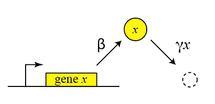
with production happening at rate $\beta$ and degradation+dilution at rate $\gamma x$. We can then write down a simple ordinary differential equation describing these dynamics:
\begin{align} \frac{dx}{dt} = \mathrm{production - (degradation+dilution)} \end{align}\begin{align} \frac{dx}{dt} = \beta - \gamma x \end{align}where
\begin{align} \gamma = \gamma_\mathrm{dilution} + \gamma_\mathrm{degradation} \end{align}A note on effective degradation rates: When cells are growing, protein is removed through both degradation and dilution. For stable proteins, dilution dominates. For very unstable proteins, whose half-life is much smaller than the cell cycle period, dilution may be negligible. In bacteria, mRNA half-lives (1-10 min, typically) are much shorter than protein half-lives. In eukaryotic cells this is not necessarily true (mRNA half-lives can be many hours in mammalian cells).
Solving for the steady state
One of the most important things we would like to know is the concentration of protein under steady state conditions. To obtain this, we set the time derivative to 0, and solve:
\begin{align} &\frac{dx}{dt} = \beta - \gamma x = 0 \\[1em] &\Rightarrow x_{\mathrm{st}} = \beta / \gamma \end{align}In other words, the protein concentration depends on the ratio of production rate to degradation rate.
Including transcription and translation as separate steps
This description is oversimplified in many ways. For example, it does not distinguish between transcription and translation, which can be important in more dynamic and stochastic contexts, as we will encounter later in the course. To do so, we can add an addition variable to represent the mRNA concentration, which is now transcribed, translated to protein, and degraded (and diluted), as shown schematically here:
These reactions can be described by two coupled differential equations for the mRNA (m) and protein (x):
\begin{align} &\frac{dm}{dt} = \beta_m - \gamma_m m, \\[1em] &\frac{dx}{dt} = \beta_p m - \gamma_p x. \end{align}Now, we can determine the steady state mRNA and protein concentrations straightforwardly, by setting both time derivatives to 0 and solving. We find:
\begin{align} &m_\mathrm{st} = \beta_m / \gamma_m, \\[1em] &x_\mathrm{st} = \frac{\beta_p m_\mathrm{st}}{\gamma_p} = \frac{\beta_p \beta_m}{\gamma_p \gamma_m}. \end{align}From this, we see that the steady state protein concentration is proportional to the product of the two synthesis rates and inversely proportional to the product of the two degradation rates.
And this gives us our first design puzzle: the cell could control protein expression level in at least four different ways, by modulating transcription, translation, mRNA degradation or protein degradation rates (or combinations of them). Are there tradeoffs between these different options? Are they all used indiscriminately or is one favored in natural contexts?
From gene expression to gene regulation - adding a repressor
Life would be simple -- perhaps too simple -- if genes were simply left "on" all the time. To make things interesting the cell has to regulate them, turning their expression levels lower or higher depending on environmental conditions and other inputs. One of the simplest ways to do this is through repressors. Repressors are proteins that can bind to specific binding sites at or near a promoter to change its activity. Often the strength of their binding is contingent on external inputs. For example, the LacI repressor normally turns off the genes for lactose utilization in E. coli. However, in the presence of lactose in the media, a modified form of lactose binds to LacI, inhibiting its ability to repress its target genes. Thus, a nutrient (lactose) can regulate expression of genes that allow the cell to use it. (For the scientific and historical saga of this seemingly simple system, we reccommend the fascinating, wonderful book "The lac operon" by B. Müller-Hill.)
In the following diagram, we label the repressor R.
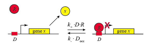
Within the cell, the repressor will bind and unbind to its target site. We assume that the expression level of the gene is lower when the repressor is bound and higher when it is unbound. The mean expression level of the gene is then proportional to the fraction of time that the repressor is unbound.
We therefore compute the "concentration" of DNA sites in occupied or unoccupied states. (Within a single cell an individual site on the DNA is either bound or unbound, but averaged over a population of cells, we can talk about the mean occupancy of the site). Let $D$ be the concentration of unoccupied promoter, $D_\mathrm{occ}$ be the concentration of occupied promoter, and $D_\mathrm{tot}$ be the total concentration of promoter, with $D_\mathrm{tot} = D + D_\mathrm{occ}$, as required by conservation of mass.
We can also assume a separation of timescales. the rates of binding and unbinding of the repressor to the DNA binding site are both often fast compared to the timescales over which mRNA and protein concentrations vary. (Careful, however, in some contexts, such as mammalian cells, this assumption need not be true.)
All we need to know is the mean concentration of unoccupied binding sites, $\frac{D}{D_\mathrm{tot}}$
\begin{align} &k_+ D R = k_- D_\mathrm{occ} \\[1em] &D_\mathrm{occ} = D_\mathrm{tot} - D \\[1em] &\frac{D}{D_\mathrm{tot}} = \frac{1}{1+R/K_d}, \end{align}where $K_d = k_ / k_+$. From this, we can write that the production rate as a function of repressor concentration:
\begin{align} \beta(R) = \beta_0 \frac{D}{D_\mathrm{tot}} = \frac{\beta_0}{1+R/K_d}. \end{align}Properties of the simple binding curve
This is our first encounter with a soon to be familiar function. Note that this function has two parameters: $K_d$ specifies the concentration of repressor at which the response is reduced to half its maximum value. The coefficient $\beta_0$ is simply the maximum expression level, and is a parameter that multiples the rest of the function.
Gene expression can be "leaky"
As an aside, we note that in real life, many genes never get repressed all the way to zero expression, even when you add a lot of repressor. Instead, there is a baseline, or "basal", expression level that still occurs. A simple way to model this is by adding an additional constant term, $\alpha$ to the expression
\begin{align} \beta(R) = \alpha_0 + \beta_0 \frac{D}{D_\mathrm{tot}} = \frac{\beta_0}{1+R/K_d}. \end{align}Given the ubiquitousness of leakiness, it is important to check that circuit behaviors do not depend on the absence of leaky expression.
Activation
Genes can be regulated by activators as well as repressors. Treating the case of activation just involves switching the state that is actively expressing from the unbound one to the one bound by the protein (now called an Activator). And, just as the binding of a repressor to DNA can be modulated by small molecule inputs, so too can the binding of the activator be modulated by binding to small molecules. In bacteria, one of many examples is the arabinose regulation system.
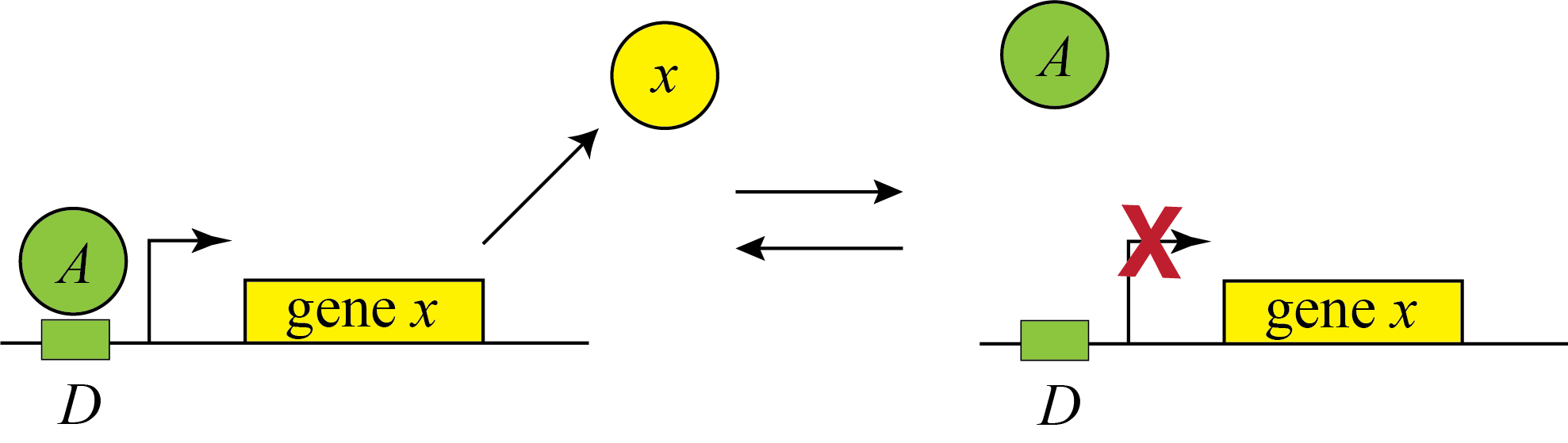
This produces the the opposite, mirror image response compared to repression, shown below with no leakage.
Activator vs. Repressor -- which to choose?
And now at last we have reached our first true 'design' question: The cell has at least two different ways to regulate a gene: using an activator or using a repressor. Which should it choose? Which would you choose if you were designing a synthetic circuit? Why? Are they completely equivalent ways to regulate a target gene? Is one better in some or all conditions? How could we know?
These questions were first posed in a study by Michael Savageau (PNAS, 1974), who tried to explain the naturally observed usage of activation and repression in bacteria. A different explanation was later developed by Shinar et al (PNAS 2004). We end the lecture with this question - try to think about when and why you would use each type of regulation!
Computing environment
%load_ext watermark
%watermark -v -p numpy,bokeh,jupyterlab