3. Big functions from small circuits
(c) 2019 Justin Bois and Michael Elowitz, except for images taken from sources where cited. This work is licensed under a Creative Commons Attribution License CC-BY 4.0. All code contained herein is licensed under an MIT license.
This document was prepared at Caltech with financial support from the Donna and Benjamin M. Rosen Bioengineering Center.

This lesson was generated from a Jupyter notebook. Click the links below for other versions of this lesson.
Design principles
- Negative autoregulation accelerates turn-on times.
- Positive feedback and ultrasensitivity enable bistability.
Key concepts
- Demand theory and error load concepts provide distinct explanations for preferential use of activation and repression.
- Protein half-lives control response times of simple gene expression units.
- Rapid protein production can accelerate response times.
- Simple feedback circuits of one or two genes can provide critical functions including accelerated responses and bistability.
Techniques
- Normalization to steady-state expression levels allows analysis of response times.
- All of the time derivatives of a system of ordinary differential equations vanish at fixed points.
- Nullclines enable identification of fixed points in multidimensional dynamical systems.
- Synthetic biology approaches enable testing of dynamics in minimal, well-controlled circuits.
Demand theory: "use it or lose it"
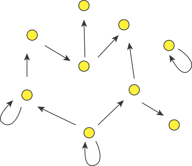
At the end of the first lecture, we asked a simple design question: When or why would you prefer to use activation or repression to regulate a gene? We know that both schemes are used, and can be used in equivalent ways:
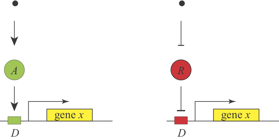
Michael Savageau posed this question in the context of bacterial metabolic gene regulation in his paper, "Design of molecular control mechanisms and the demand for gene expression" (PNAS, 1977). He focused on "demand" as a critical factor that influences the choice of activation or repression. Demand can be defined as the fraction of time that the gene is needed at the high end of its regulatory range in the cells natural environments. Savageau made the empirical observation that high demand genes are more frequently regulated by activators, while low demand genes are more often regulated by repressors.
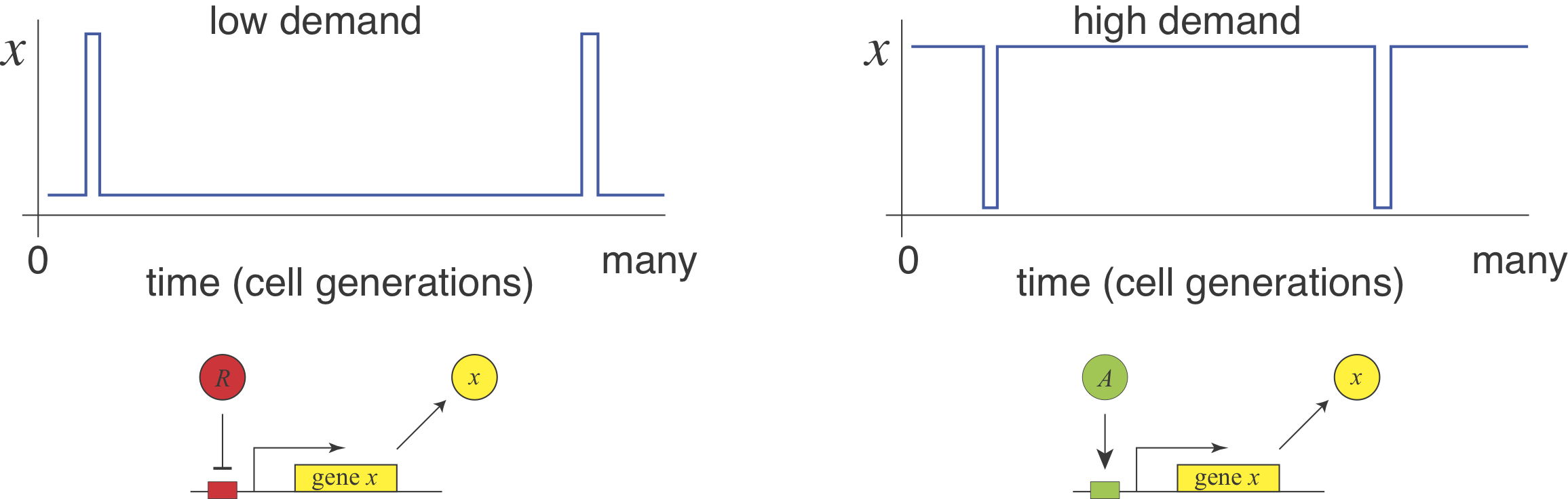
He suggested that this relationship (somewhat counterintuitively) could be explained by a "use it or lose it" rule of evolutionary selection. A high demand gene controlled by an activator needs the activator to be on most of the time. Mutations that eliminate the activator would therefore be selected against in most conditions. By contrast, if the same high demand system were regulated by a repressor, in most conditions, there would be no selection against mutations that removed the repressor, more readily permitting evolutionary loss of the system. This reasoning assumes no direct fitness advantage for either regulation mode, just a difference in their likelihood of evolutionary loss.
In a 2009 PNAS paper, Gerland and Hwa formulated and analyzed a model to explore these ideas mathematically. They showed that the "use it or lose it" principle dominates when timescales of switching between low and high demand environments are long and populations are small. (However, the same model could select for the opposite demand rule in other regimes.)
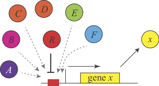
Shinar, et al. introduced a completely different explanation for the demand rules, based on the concept of "error load". The authors assumed that "naked" DNA binding sites, which are not bound to proteins, are susceptible to non-specific binding of transcription factors, which is assumed to impose a low, but non-zero fitness cost by inappropriately perturbing gene expression. Keeping these sites occupied most of the time minimizes the chances of such errors. This explanation also predicts that a high demand gene should preferentially use an activator since this arrangement minimizes unoccupied binding sites. Conversely, a low demand gene would preferentially use repression to maintain the binding site in an occupied state under most conditions. This argument can be generalized to other examples of seemingly equivalent regulatory systems and is described in Uri Alon's book.
Remarkably, we still lack definitive experimental evidence to fully resolve this fundamental design question. Can you think of an experimental way to test one of these models?
Dynamics: protein stability determines the response time to a change in gene expression
We now return to simple gene regulation circuits. So far, we have focused on steady states. However, many of the most important and fascinating biological systems change dynamically, even in constant environmental conditions.
The most basic dynamic question one can ask about a gene is how rapidly it can switch from one level of protein to a new level after a sudden increase or decrease in gene expression.
Starting with our basic equation for gene expression, and neglecting the mRNA level for the moment, we write:
\begin{align} \frac{\mathrm{d}x}{\mathrm{d}t} = \beta - \gamma x \end{align}Consider a simple situation in which the gene has been off for a long time, so that $x(t=0)=0$ and then is suddenly turned on at $t=0$. The solution to this simple differential equation is:
\begin{align} x(t) = \frac{\beta }{\gamma} (1-e^{-\gamma t}) \end{align}Thus, the parameter that determines the response time is $\gamma$, the degradation+dilution rate of the protein. We define the response time to be $\gamma^{-1}$, which is the time it takes for the concentration to rise to a factor of $1-\mathrm{e}^{-1}$ of its steady state value. We show the response time as a dot on the plot below.
How can we speed up responses?
So far, it seems like the cell's ability to modulate the concentration of a stable protein is quite limited, apparently requiring multiple cell cycles for both increases and decreases. This seems rather pathetic for a billion year old creature. You might think you could up-regulate the protein level faster by cranking up the promoter strength (increasing $\beta$). Indeed, this could allow the cell to hit a specific threshold faster. However, it would also increase the final steady state level ($\beta/\gamma$), and therefore leave the timescale over which the system reaches its new steady-state unaffected.
One simple and direct way to speed up the response time of the protein is to destabilize it, increasing $\gamma$. This strategy pays the cost of a "futile cycle" of protein synthesis and degradation to provide a benefit in terms of the speed with which the regulatory system can reach a new steady state. It is useful to normalize these plots by their steady states in order to focus on response times independently of steady states, as shown in the second plot below. (This is a reasonable comparison because there are many mutations that alter the expression level of a gene; this property can be optimized by evolution independently of the regulatory feedback architecture).
Design principle: Increased turnover speeds up the response time of a gene expression system, at the cost of additional protein synthesis and degradation.
Negative autoregulation is prevalent in natural circuits
Most bacterial proteins, transcription factors in particular, are stable. Do they use other mechanisms to accelerate response times?
Empirically, we find that a large fraction of repressors repress their own expression.
In fact, we can consider autoregulation to be a network motif, defined as a regulatory pattern that is statistically over-represented in natural networks (circuits) compared to random networks. To see this, it is useful to think of the transcriptional regulatory network of an organism as a 'graph' consisting of nodes and directed edges (arrows). In bacteria, each node represents an operon, while each arrow represents regulation of the target operon (tip of the arrow) by a transcription factor in the originating node (base of the arrow), as shown schematically here.
The transcriptional regulatory network of E. coli has been mapped (see RegulonDB). It contains ≈424 operons (nodes), ≈519 transcriptional regulatory interactions (arrows), involving ≈116 transcription factors. If the target of each arrow was chosen randomly, the probability of any given arrow being autoregulatory is low (≈1/424). One might expect only about one such event in the entire network. However, ≈40 such autoregulatory arrows are observed. Autoregulation thus appears to be over-represented.
(If we further consider the "sign" of the arrow, with "+" representing activation and "-" representing repression, it turns out that there are 32 negative autoregulatory operons and 8 positive autoregulatory ones. We will discuss both types.)
Motif principle: Given that autoregulation is so heavily over-represented, one can ask what function might it provide. This is analogous to identifying statistically over-represented sequence motifs within the genome and analyzing their functional behaviors. We will discuss motifs further in the next lecture.
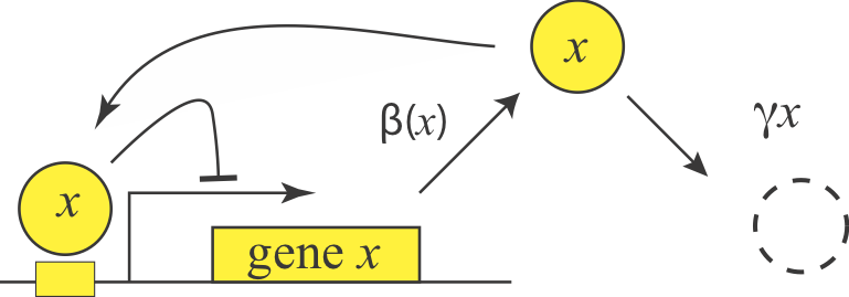
Negative autoregulation accelerates response times
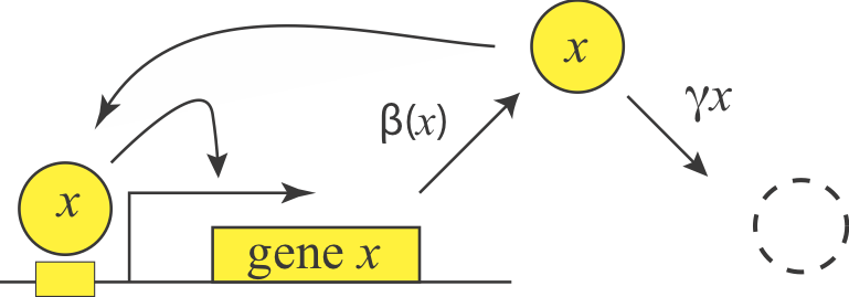
Given its prevalence, it is natural to ask what function or functions negative autoregulation provides for the cell. We start by writing down a simple differential equation for the concentration of the repressor, $x$:
\begin{align} \frac{\mathrm{d}x}{\mathrm{d}t}=\frac{\beta}{1+x/K_d} - \gamma x \end{align}What happens when the operon is suddenly turned "on?" We will consider the limit in which the autoregulation is "strong", i.e. where $\beta/\gamma \gg K_d$, so the gene can, at maximal expression level, produce enough protein to fully repress itself.
After the gene turns on, starting from an "off" initial condition, it initially builds up linearly, at rate $\beta$, until its concentration is high enough to shut its own production off, $x \sim K_d$, going something like this:
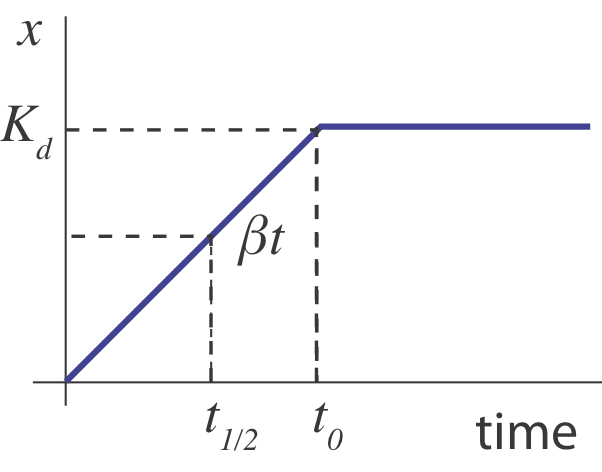
In this sketch, we can see that we might expect that the half-time, $t_{1/2}$ for turning on should occur when $\beta t \approx K_d / 2$, i.e. at $t \approx K_d/2 \beta$. But this is only an approximation. A more complete treatement, in Rosenfeld et al. (JMB 2002) shows that in the limit of strong negative autoregulation the dynamics approach the following expression: $x(t) = x_\mathrm{st} \sqrt{1-e^{-2 \gamma t}}$, where $x_\mathrm{st}$ denotes the steady-state expression level.
We can also explore the system using numerical integration.
Not surprisingly, adding negative autoregulation reduced the steady-state expression level. However, it also had a second effect: accelerating the approach to steady state. In the right-hand plot we include the limiting analytical solution from Rosenfeld et al. for comparison.
Negative autoregulation has accelerated the dynamics by about 5-fold compared to the unregulted system.
Note that this acceleration occurs when we turn the gene on, but not when we turn it off. If we suddenly change $\beta$ to 0, then the dynamics are governed by $\mathrm{d}x/\mathrm{d}t = -\gamma x$ irrespective of which architecture we use.
Can this acceleration be observed experimentally? To find out, Rosenfeld et al. engineered a simple synthetic system based on a bacterial repressor called TetR, fused to a fluorescent protein for readout, and studied its turn-on dynamics in bacterial populations.
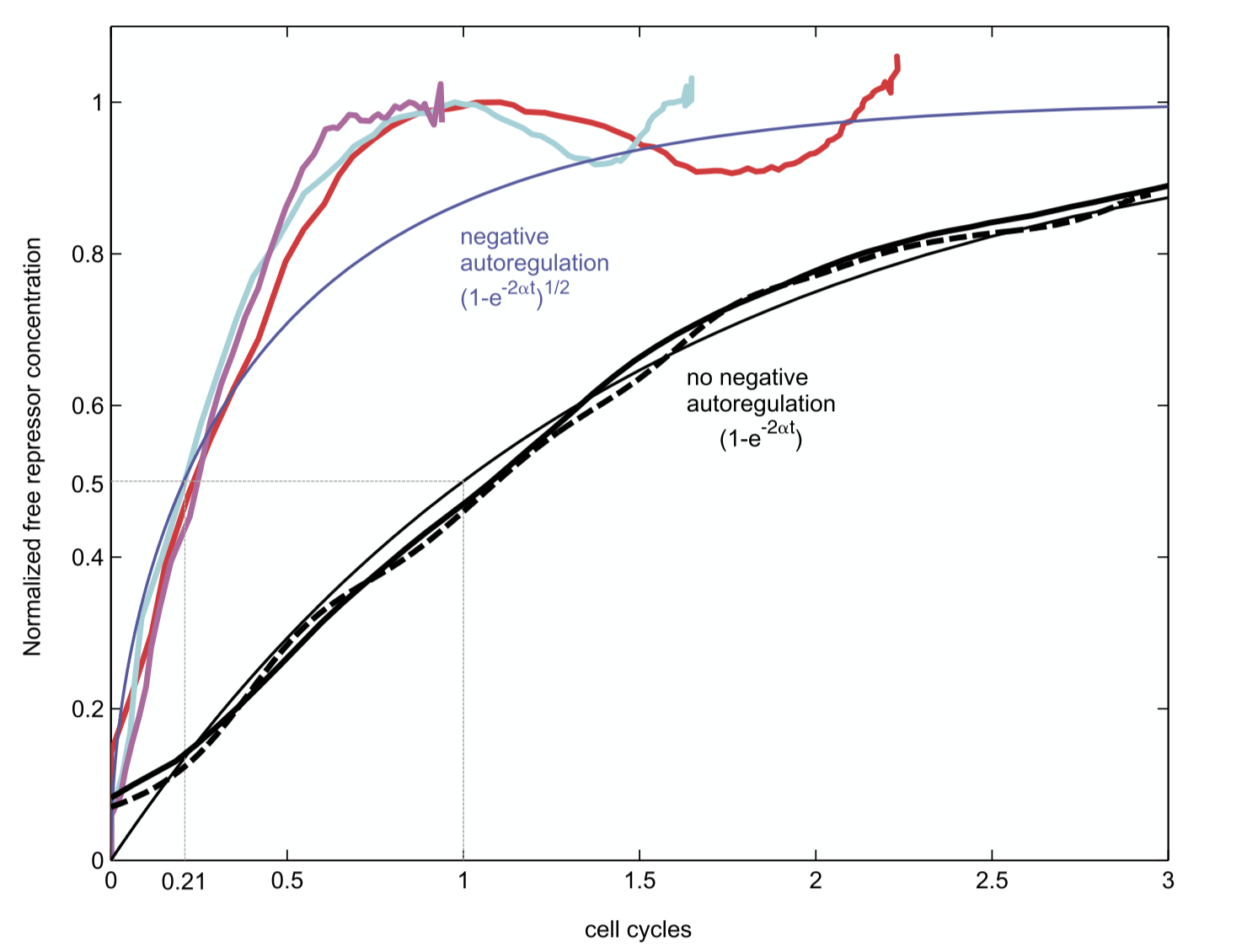
Interestingly, these dynamics showed the expected acceleration, as well as some oscillations around steady-state, which may be explained by time delays in the regulatory system.
To conclude this section: We now have identified another simple design principle: Negative autoregulation speeds the response time of a transcription factor.
Negative autoregulation can have additional functions beyond acceleration. Using similar synthetic approaches, negative autoregulation was shown to reduce stochastic cell-cell variability ("noise") in gene expression (Becskei and Serrano, Nature, 2000).
Positive autoregulation enables bistability
Having examined negative autoregulation, we can also ask what functions positive autoregulation, which is also prevalent in natural circuits, might provide.
We can represent a positive autoregulatory circuit with the following simple equation:
\begin{align} \frac{\mathrm{d}x}{\mathrm{d}t} = \frac{\beta x^n} {x^n + K^n} - \gamma x \end{align}To think about what this circuit can do, let's plot the two terms on the right hand side (production rate and removal rate) versus $x$. We will start by considering a relatively high Hill coefficient of $n=4$.
Wherever production rate = degradation rate, we have a fixed point. For these parameters, there are three fixed points. These points differ in their stability. The one in the middle is unstable, while the two on the ends are stable. The easiest way to see this is to notice that between the first and second fixed points removal rate > production rate, and hence x will decrease, while between the second and third fixed points, production exceeds removal, and x will increase.
Since this system has two stable fixed points, we can describe it as bistable. As long as noise or other perturbations are not too strong, the cell can happily remain at either a low or high value of x.
Bistability is a special case of the more general phenomenon of multistability, which is one of the most important properties in biology, underlying the ability of a single genome to produce a vast array of distinct cell types in a multicellular organism. This simple analysis shows us immediately that a single gene positive feedback loop can be sufficient to generate bistability!
However, positive feedback by itself is not enough. We also need an ultrasensitive response to $x$. (In the context of the Hill function, ultrasensitivity can be defined simply as $n>1$). If we reduce the Hill coefficient to 1, keeping other parameters the same, you can see that we now have only a single stable fixed point (and one unstable fixed point at $x=0$).
Furthermore, ultrasensitivity is also not enough. Bistability in this system further requires tuning of different rate constants. For example, consider what happens for varying values of $\gamma$. (Here, I've set a very high value of $n=10$ just to focus on how the role of $\gamma$)
Note that with just a two-fold higher value of $\gamma=2$ (upper orange line), we lose the last two fixed points, giving us a monostable system that just remains, sadly, at 0, totally unable to activate itself. Based on considerations like this, we can see that positive autoregulatory feedback and ultrasensitivity do not, in general, guarantee bistability, though they can provide it. That leads us to the design principle: Positive, ultrasensitive autoregulation enables bistability.
The toggle switch: a two-gene positive feedback system
In natural circuits positive feedback loops are often observed among multiple regulators rather than just a single autoregulatory transcription factor. For example, the "genetic switch" in phage lambda involves reciprocal repression of the cro repressor by the $\lambda$ repressor, and vice versa (see Mark Ptashne's classic book, A genetic switch). This arrangement allows the phage to remain in the dormant "lysogenic" state or switch to a "lytic" state in which it replicates and eventually lyses the host cell to infect other cells.
In 2000, Gardner and Collins designed, constructed, and analyzed a synthetic version of this feedback loop, termed the toggle switch, and showed that it could similarly exhibit bistability. Here is a simple diagram of the general design.
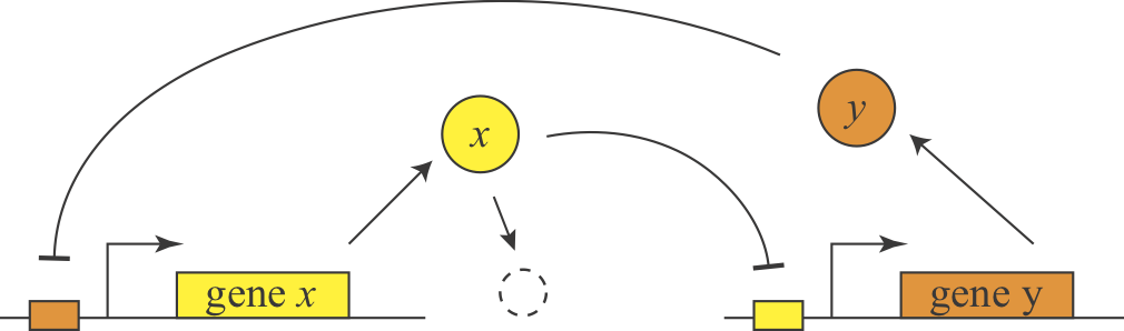
To analyze this two-repressor feedback loop, we can write down a simplified model for the levels of both the $x$ and $y$ proteins, both having the same Hill coefficient, $n$.
\begin{align} &\frac{dx}{dt} = \frac{\beta_x}{1 + (y/k_y)^n} - \gamma_x x,\\[1em] &\frac{dy}{dt} = \frac{\beta_y}{1 + (x/k_x)^n} - \gamma_y y. \end{align}We nondimensionalize by taking $\beta_x \leftarrow \beta_x/\gamma_x k_x$, $\beta_y \leftarrow \beta_y/\gamma_y k_y$, $x \leftarrow x/k_x$, $y \leftarrow y/k_y$, $t \leftarrow \gamma_x t$, and $\gamma = \gamma_y/\gamma_x$. We can now see that the behavior of the system really depends only on (a) the strengths of the two promoters, (b) the relative timescales of the two proteins, and (c) the sensitivity of the response (Hill coefficient):
\begin{align} \frac{dx}{dt} &= \frac{\beta_x}{1 + y^n} - x,\\[1em] \gamma^{-1}\,\frac{dy}{dt} &= \frac{\beta_y}{1 + x^n} - y. \end{align}A great way to analyze a two-dimensional system like this is by computing the nullclines, which are defined by setting each of the time derivatives equal to zero.
\begin{align} x\text{ nullcline: }& x = \frac{\beta_x}{1 + y^n}, \\[1em] y\text{ nullcline: }& y= \frac{\beta_y}{1 + x^n}. \end{align}Wherever these two lines cross, one has a fixed point. The stability of that fixed point can be determined by linear stability analysis, which we will introduce in a later lesson. For now, we will plot the two nullclines and investigate their behavior by varying the dimensionless parameters $\beta_x$ and $\beta_y$, as well as the Hill coefficient $n$. The plot we show below is interactive, including in the HTML rendering of this lesson.
You can investigate the nullclines by playing with the sliders. For $\beta_x = \beta_y = 10$ and $n = 4$, we clearly have three crossings of the nullclines, giving one unstable (the one in the middle) and two stable (the ones on the ends) fixed points.
Try sliding the $n$ slider. As you move $n$ down, you can see that one can still obtain bistability at lower Hill coefficients, but one can see it becomes a more delicate balancing act where the values of $\beta_x$ and $\beta_y$ need to be large and close in magnitude. Bistablity is lost completely at $n=1$, where the system becomes monostable.
Even at higher Hill coefficients, the strengths of the promoters must still be balanced. If we have widely varying values of $\beta_x$ and $\beta_y$, we again have monostability. You can see this by setting $\beta_x = 10$, $\beta_y = 1.5$, and $n = 5$ with the sliders.
Thus, as with the single gene autoregulatory positive feedback loop, ultrasensitivity is necessary but not sufficient for bistability. Later in the course, we will further analyze this system and its stability, learning how to further characterize dynamical systems beyond their nullclines.
Discussion question: What are the advantages of the two-gene toggle switch compared to the single gene positive autoregulation circuit?
Summary
- Protein degradation and dilution rates determine (and limit) the switching speed of a simple transcriptinally regulated gene.
- Design principle: Negative autoregulation accelerates turn-on of a transcription factor.
- Design principle: Positive, ultrasensitive autoregulation generates bistability.
- Even simple circuits of 1 or 2 genes can generate interesting functional capabilities.
- Synthetic circuits can be used to test the functions of simple circuits in living cells.
This is our first foray into the analysis of dynamical systems. As we continue to work with dynamical systems, Strogatz's book is a great introduction, and includes discussion on using nullclines in the analysis.
Computing environment
%load_ext watermark
%watermark -v -p numpy,scipy,bokeh,jupyterlab