9. Delay oscillators
(c) 2019 Justin Bois and Michael Elowitz. With the exception of pasted graphics, where the source is noted, this work is licensed under a Creative Commons Attribution License CC-BY 4.0. All code contained herein is licensed under an MIT license.
This document was prepared at Caltech with financial support from the Donna and Benjamin M. Rosen Bioengineering Center.

This lesson was generated from a Jupyter notebook. Click the links below for other versions of this lesson.
We continue our discussion of oscillators by considering a very simple oscillator, perhaps even simpler than the repressilator. We will consider a single-component circuit with negative feedback with delay. The basic idea has been put forward many times, notably by Julian Lewis in 200300534-7), describing transcriptional delay.
A simple delay oscillator
For the simplest picture, consider an autoinhibitory gene. The inhibition of transcription if realized by the protein product, which takes a while to be made after transcription. So, there is a time delay between the onset of production of the mRNA transcript and the effect of self-repression. We will call this time delay $\tau$. So, we can write a differential equation describing the dynamics of expression of this gene (which we will call X) as
\begin{align} \frac{\mathrm{d}x}{\mathrm{d}t} = \frac{\beta}{\displaystyle{1+\left(\frac{x(t-\tau)}{k}\right)^n}} - \gamma x. \end{align}In other words, we are stating that the expression of X at time $t$ is dependent on its expression level at time $t - \tau$. This is a delay differential equation (DDE).
Doing our usual nondimensionalization, setting $\beta \leftarrow \beta/\gamma$, $t\leftarrow \gamma t$, $x\leftarrow x/k$, and $\tau \leftarrow\gamma \tau$, we have
\begin{align} \frac{\mathrm{d}x}{\mathrm{d}t} = \frac{\beta}{1+(x(t-\tau))^n} - x. \end{align}We can solve this numerically to get oscillations, which we will do momentarily.
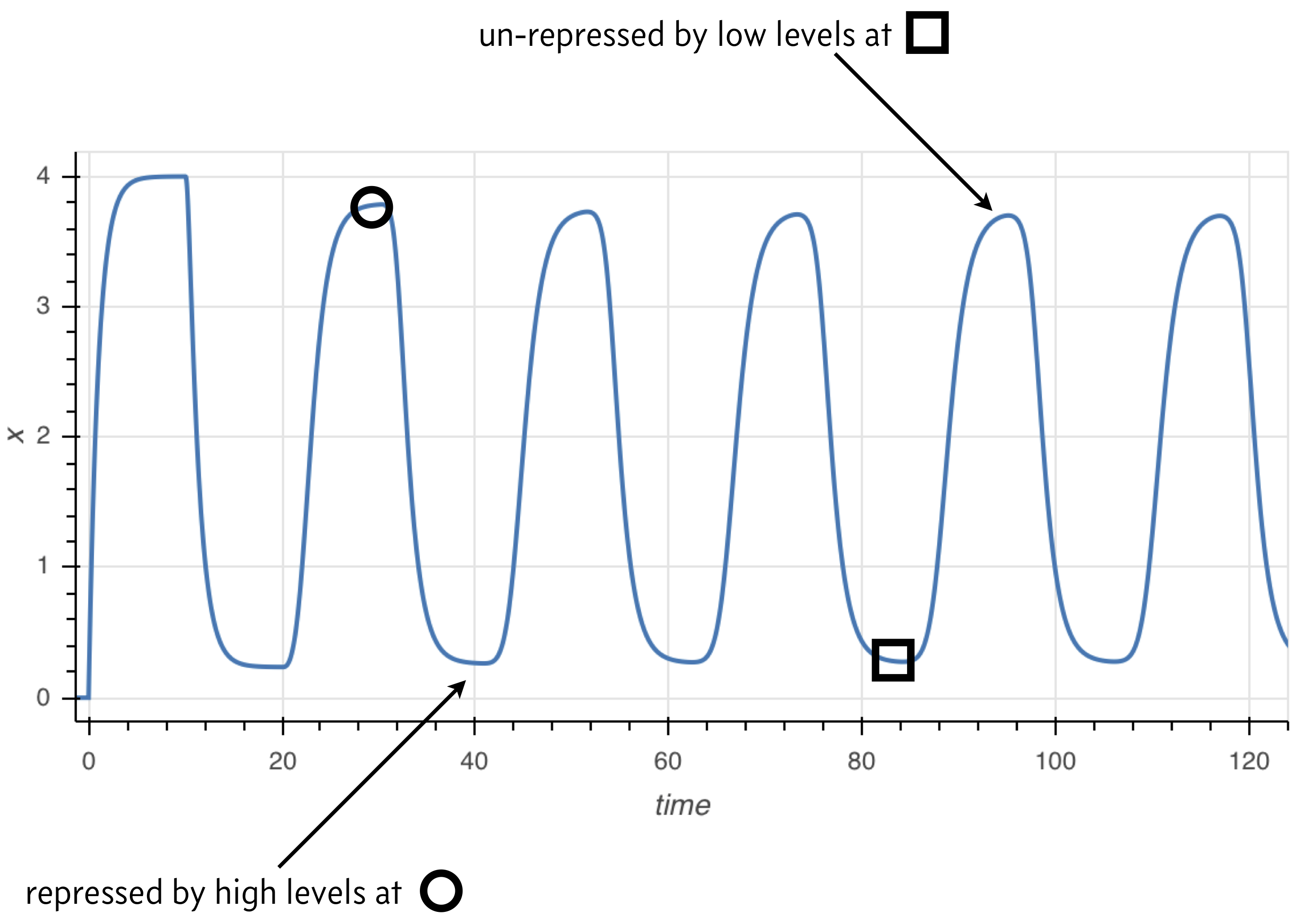
The principle behind the presence of oscillations is simple, and illustrated in the image below. Because the rate of expression is determined by past protein levels, high expression occurs when protein levels were low in the past and low expression occurs when protein levels were high in the past.
Numerical solution of DDEs
In general, we may write a system of DDEs as
\begin{align} \frac{\mathrm{d}\mathbf{u}}{\mathrm{d}t} = &= \mathbf{f}(t, \mathbf{u}(t), \mathbf{u}(t-\tau_1), \mathbf{u}(t-\tau_2), \ldots, \tau_n), \end{align}where $\tau_1, \tau_2, \ldots, \tau_n$ are the delays with $\tau_1 < \tau_2 < \ldots < \tau_n$. We define the longest delay to be $\tau_n = \tau$ for notational convenience. If we wish to have a solution for time $t \ge t_0$, we need to specify initial conditions that go sufficiently far back in time,
\begin{align} y(t) = y_0(t) \text{ for }t_0-\tau < t \le t_0. \end{align}The approach we will take is the method of steps. Given $y_0(t)$, we integrate the differential equations from time $t_0$ to time $t_0 + \tau$. We store that solution and then use it to integrate again from time $t_0+\tau$ to time $t_0 + 2\tau$. We continue this process until we integrate over the desired time span.
Because we need to access $y(t-\tau_i)$ at time $t$, and $t$ can be arbitrary, we often need an interpolation of the solution from the previous time steps. We will use SciPy's functional interface for B-spline interpolation, using the scipy.interpolate.splrep() and scipy.interpolate.splev() functions.
We write the function below to solve DDEs with similar call signature as scipy.integrate.odeint().
ddeint(func, y0, t, tau, args=(), y0_args=(), n_time_points_per_step=200)
The input function has a different call signature than odeint() because it needs to allow for a function that computes the values of y in the past. So, the call signature of the function func giving the right hand side of the system of DDEs is
func(y, t, y_past, *args)
Furthermore, instead of passing in a single initial condition, we need to pass in a function that computes $y_0(t)$, as defined for initial conditions that go back in time. The function has call signature
y0(t, *y0_args)
We also need to specify tau, the longest time delay in the system. Finally, in addition to the additional arguments to func and to y0, we specify how many time points we wish to use for each step to build our interpolants. Note that even though we specify tau in the arguments of ddeint(), we still need to explicitly pass all time delays as extra args to func. This is because we could in general have more than one delay, and only the longest is pertinent for the integration.
def ddeint(func, y0, t, tau, args=(), y0_args=(), n_time_points_per_step=200):
    """Integrate a system of delay differential equations.
    """
    t0 = t[0]
    y_dense = []
    t_dense = []

    # Past function for the first step
    y_past = lambda t: y0(t, *y0_args)

    # Integrate first step
    t_step = np.linspace(t0, t0+tau, n_time_points_per_step)
    y = scipy.integrate.odeint(func, y_past(t0), t_step, args=(y_past,)+args)

    # Store result from integration
    y_dense.append(y[:-1, :])
    t_dense.append(t_step[:-1])

    # Get dimension of problem for convenience
    n = y.shape[1]

    # Integrate subsequent steps
    j = 1
    while t_step[-1] < t[-1] and j < 100:
        # Make B-spline
        tck = [scipy.interpolate.splrep(t_step, y[:,i]) for i in range(n)]

        # Interpolant of y from previous step
        y_past = lambda t: np.array([scipy.interpolate.splev(t, tck[i])
                                         for i in range(n)])

        # Integrate this step
        t_step = np.linspace(t0 + j*tau, t0 + (j+1)*tau, n_time_points_per_step)
        y = scipy.integrate.odeint(func, y[-1,:], t_step, args=(y_past,)+args)

        # Store the result
        y_dense.append(y[:-1, :])
        t_dense.append(t_step[:-1])

        j += 1

    # Concatenate results from steps
    y_dense = np.concatenate(y_dense)
    t_dense = np.concatenate(t_dense)

    # Interpolate solution for returning
    y_return = np.empty((len(t), n))
    for i in range(n):
        tck = scipy.interpolate.splrep(t_dense, y_dense[:,i])
        y_return[:,i] = scipy.interpolate.splev(t, tck)

    return y_return
Now that we have a function to solve DDEs, let's solve the simple delay oscillator we hand.
# Right hand side of simple delay oscillator
def delay_rhs(x, t, x_past, beta, n, tau):
    return beta / (1 + x_past(t-tau)**n) - x

# Initially, we just have no gene product
def x0(t):
    return 0

# Specify parameters (All dimensionless)
beta = 4
n = 2
tau = 10

# Time points we want
t = np.linspace(0, 200, 400)

# Perform the integration
x = ddeint(delay_rhs, x0, t, tau, args=(beta, n, tau))

# Plot the result
p = bokeh.plotting.figure(plot_width=600,
                          plot_height=300,
                          x_axis_label='time',
                          y_axis_label='x')
p.line(t, x[:,0], line_width=2)

bokeh.io.show(p)
The ddeint() function is available as biocircuits.ddeint() package for future use.
An example of delay in a biological circuit
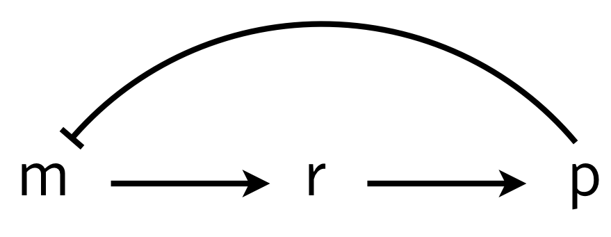
To investigate how molecular details can give rise to delay (which in turn can give oscillations), we consider a multistep process of the production and action of a repressor. The delay in transcriptional regulation in real cells comes from processes such as translation, trans-nuclear transport, etc. We will consider a simple version of this, shown below, in which $r$ is some intermediate state en route to functioning protein.
We can write the dynamics as
\begin{align} \frac{\mathrm{d}m}{\mathrm{d}t} &= \frac{\beta_{m}}{1 + (p/k)^n} - \gamma_m m,\\[1em] \frac{\mathrm{d}r}{\mathrm{d}t} &= \beta_{r} m - \gamma_r r,\\[1em] \frac{\mathrm{d}p}{\mathrm{d}t} &= \beta_{p} r - \gamma_{p} p, \end{align}where for simplicity we have assumed mass action type kinetics for all processes other than repression. These equations can be nondimensionalized by renaming parameters and variables as $r \leftarrow \gamma_m t$, $p \leftarrow p/k$, $m \leftarrow \beta_{r}\beta_{p} m/\gamma_m^2 k$, $r \leftarrow \beta_{p} r/\gamma_m k$, $\beta \leftarrow \beta_{m} \beta_{r} \beta_{p}/\gamma_m^2 k$ and $\gamma \leftarrow \gamma_{p}/\gamma_m$ to give
\begin{align} \frac{\mathrm{d}m}{\mathrm{d}t} &= \frac{\beta}{1 + p^n} - m,\\ \frac{\mathrm{d}r}{\mathrm{d}t} &= m - r,\\ \frac{\mathrm{d}p}{\mathrm{d}t} &= r - \gamma p. \end{align}There is a single fixed point $(m_0, r_0, p_0)$ for this system,
\begin{align} m_0 &= r_0 = \gamma p_0,\\ \frac{\beta}{\gamma} &= p_0(1+p_0^n). \end{align}We can perform linear stability analysis about this fixed point, just as we did in for the repressilator.
\begin{align} \frac{\mathrm{d}}{\mathrm{d}t}\begin{pmatrix} \delta m \\ \delta r \\ \delta p \end{pmatrix} = \mathsf{A}\cdot\begin{pmatrix} \delta m \\ \delta r \\ \delta p \end{pmatrix}, \end{align}with
\begin{align} \mathsf{A} = \begin{pmatrix} -1 & 0 & -a \\ 1 & -1 & 0 \\ 0 & 1 & -\gamma \end{pmatrix}, \end{align}where
\begin{align} a = \frac{\beta n p_0^{n-1}}{(1+p_0^n)^2} = \frac{\gamma n p_0^n}{1+p_0^n}. \end{align}To find the eigenvalues, we write the characteristic polynomial as
\begin{align} -(1+\lambda)^2(\gamma+\lambda) - a = -\lambda^3 - (2+\gamma)\lambda^2 - (1+2\gamma)\lambda -\gamma - a = 0. \end{align}This polynomial has no positive real roots and either one or three negative real roots according to the Descartes Sign Rule. We are interested in the case where we have one negative real root and two complex conjugate roots. If the real part of these complex conjugate roots is positive, we have an oscillatory instability.
We can compute the eigenvalues of the linear stability matrix for various values of $\beta$ and $\gamma$ for fixed Hill coefficient $n$. We will take a "brute force" approach and grid up $\beta$-$\gamma$ space and compute the eigenvalues for each set of parameter values and determine if that point is stable or not. We can then display the linear stability diagram as an image, where a pixel is light colored in a stable region and dark colored in an unstable region.
def fixed_point(beta, gamma, n):
    """Computes fixed point the m⟶r⟶p autorepression system.
    Uses np.roots because it has better convergence properties than
    scipy.optimize.fixed_point for integer n.
    """
    coeffs = np.zeros(n+1)
    coeffs[0] = 1
    coeffs[-2] = 1
    coeffs[-1] = -beta / gamma
    p_0 = np.roots(coeffs)

    return p_0[(p_0.imag == 0) & (p_0 > 0)].real[0]


def lin_stab(beta, gamma, n):
    """Returns True if delay system is linearly stable and False
    otherwise.
    """
    p_0 = fixed_point(beta, gamma, n)

    # Linear stability matrix
    a = gamma * n * p_0**n / (1 + p_0**n)
    L = np.array([[-1, 0, -a],
                  [1, -1, 0],
                  [0, 1, -gamma]])

    # Compute eigenvalues
    lam = np.linalg.eigvals(L)

    return (lam.real < 0).all()

# Ultrasensitivity
n = 10

#
beta_vals = np.logspace(0, 4, 400)
gamma_vals = np.logspace(-1, 2, 400)

# Compute the linear stability diagram
stab = np.empty((len(beta_vals), len(gamma_vals)))
for i, beta in enumerate(beta_vals):
    for j, gamma in enumerate(gamma_vals):
        stab[i,j] = lin_stab(beta, gamma, n)

# Plot the result (shaded region has oscillatory instability)
p = bokeh.plotting.figure(plot_height=300,
                          plot_width=350,
                          x_axis_label='γ',
                          y_axis_label='β',
                          x_axis_type='log',
                          y_axis_type='log',
                          x_range=bokeh.models.Range1d(0.1, 100),
                          y_range=bokeh.models.Range1d(1, 10000))
p.image([stab], x=0.1, y=1, dw=100, dh=10000, palette='Greys3', alpha=0.5)
p.text(x=0.45, y=100, text=['unstable'])
p.text(x=10, y=2, text=['stable'])

bokeh.io.show(p)
Importantly, we see that we must have very high ultrasensitivity ($n$ about 9 or 10) to get oscillatory instabilities for reasonable values of $\beta$ and $\gamma$. Furthermore, the sliver of parameter space that gives an oscillatory instability is small. For such a simple mechanism for delay, the presence of oscillations are not robust to parameter values and high sensitivity is necessary.
To gain better insights on how the delay affects stability, we will consider the stability of the simple picture described by the DDE we first proposed and solved numerically.
\begin{align} \frac{\mathrm{d}x}{\mathrm{d}t} = \frac{\beta}{1+(x(t-\tau))^n} - x. \end{align}First, we lay the groundwork for linear stability of delayed differential equations.
Linear stability analysis of a delayed differential equation
Consider a system of delay differential equations,
\begin{align} \frac{\mathrm{d}\mathbf{u}}{\mathrm{d}t} &= \mathbf{f}(\mathbf{u}(t), \mathbf{u}(t-\tau)). \end{align}Here, we have written that the time derivative explicitly depends on the value of $\mathbf{u}$ at the present time and also at some time $\tau$ time units ago in the past. A steady state of the delay differential equations, $\mathbf{u}_0$ satisfies $\mathbf{u}_0(t) = \mathbf{u}_0(t-\tau) \equiv \mathbf{u}_0$ by the definition of a steady state. So, the steady state $\mathbf{u}_0$ satisfies $\mathbf{f}(\mathbf{u_0}, \mathbf{u}_0) = 0$. We will perform a linear stability analysis about this steady state.
To linearize, we now have the $\mathbf{f}$ is a function of two sets of variables, present and past $\mathbf{u}$. We then write a Taylor series expansion with respect to both of these variables to linearize.
\begin{align} \mathbf{f}(\mathbf{u}(t), \mathbf{u}(t-\tau)) \approx \mathbf{f}(\mathbf{u}, \mathbf{u}_0) + \mathsf{A}\cdot(\mathbf{u}(t) - \mathbf{u}_0) + \mathsf{A}_{\tau}\cdot(\mathbf{u}(t-\tau) - \mathbf{u}_0), \end{align}where
\begin{align} \mathsf{A} = \begin{pmatrix} \frac{\partial f_1}{\partial u_1(t)} & \frac{\partial f_1}{\partial u_2(t)} & \cdots \\[0.5em] \frac{\partial f_2}{\partial u_1(t)} & \frac{\partial f_2}{\partial u_2(t)} & \cdots \\ \vdots & \vdots & \ddots \end{pmatrix} \end{align}and
\begin{align} \mathsf{A}_{\tau} = \begin{pmatrix} \frac{\partial f_1}{\partial u_1(t-\tau)} & \frac{\partial f_1}{\partial u_2(t-\tau)} & \cdots \\[0.5em] \frac{\partial f_2}{\partial u_1(t-\tau)} & \frac{\partial f_2}{\partial u_2(t-\tau)} & \cdots \\ \vdots & \vdots & \ddots \end{pmatrix}, \end{align}where all derivatives in both matrices are evaluated at $\mathbf{u}(t) = \mathbf{u}(t-\tau) = \mathbf{u}_0$. Defining $\delta\mathbf{u} = \mathbf{u} - \mathbf{u}_0$, our linearized differential equations are
\begin{align} \frac{\mathrm{d}\delta\mathbf{u}}{\mathrm{d}t} = (\mathsf{A} + \mathsf{A}_{\tau})\cdot \delta\mathbf{u}. \end{align}To solve the linear system, we insert the ansatz, $\delta\mathbf{u} = \mathbf{w}\,\mathrm{e}^{\lambda t}$, giving
\begin{align} \lambda \mathrm{e}^{\lambda t}\,\mathbf{w} = \mathsf{A}\cdot\mathbf{w}\,\mathrm{e}^{\lambda t} + \mathsf{A}_{\tau}\cdot \mathbf{w}\,\mathrm{e}^{\lambda (t-\tau)}, \end{align}or, upon simplifying,
\begin{align} \lambda \mathbf{w} = (\mathsf{A} + \mathrm{e}^{-\lambda \tau} \mathsf{A}_{\tau})\cdot \mathbf{w}. \end{align}So, $\lambda$ is an eigenvalue and $\mathbf{w}$ the corresponding eigenvector for the matrix $(\mathsf{A} + \mathrm{e}^{-\lambda \tau} \mathsf{A}_{\tau})$. In general, there are infinitely many values of $\lambda$. Nonetheless, if we can show that the real part of all possible values of $\lambda$ is less than zero, then the fixed point is stable. Otherwise, if the real part of any values of $\lambda$ are positive, the fixed point is locally unstable. If $\lambda$ has an imaginary part for the eigenvalues where the real part is positive, the instability is oscillatory.
Linear stability analysis of delayed autorepression
We consider now the simple case of an autorepressor with delay.
\begin{align} \frac{\mathrm{d}x(t)}{\mathrm{d}t} = \frac{\beta}{1 + (x(t-\tau))^n} - x(t). \end{align}The steady state $x_0$ is given by setting the time derivative to zero,
\begin{align} \beta = x_0(1+x_0^n). \end{align}The $x_0$ that satisfies this equality is unique because the right hand is monotonically increasing from zero, so it only crosses a value of $\beta$ once. So, we will consider the stability of this unique steady state.
We linearize the right hand side of the ODE around the fixed point. The matrices $\mathsf{A}$ and $\mathsf{A}_{\tau}$ are scalars in this case because we have a single species. Remember that the eigenvalue of a scalar is just the scalar itself. So, we have
\begin{align} &\mathsf{A} = -1 \\[1em] &\mathsf{A}_{\tau} = -\frac{\beta n x_0^{n-1}}{(1+x_0^n)^2} = -\frac{nx_0^n}{1+x_0^n} \equiv -a_{\tau}, \end{align}where we have defined $a_{\tau}$ for convenience. Thus, our characteristic equation is
\begin{align} \lambda = -1 - a_{\tau}\mathrm{e}^{-\lambda \tau}. \end{align}There are infinitely many $\lambda$ that satisfy this equation in general. Nonetheless, we can still make progress. We write $\lambda = a + ib$, where $a$ is the real part at $b$ is the imaginary part. Then, the characteristic equation is
\begin{align} a + ib = -a_{\tau} \mathrm{e}^{-a\tau} \mathrm{e}^{-ib\tau} - 1 = -a_{\tau}\mathrm{e}^{-a\tau}(\cos b\tau - i\sin b\tau) - 1. \end{align}This can be written as two equations by equating the real and imaginary parts of both sides of the equality.
\begin{align} a &= -(1+a_{\tau} \mathrm{e}^{-a\tau} \cos b\tau ) \\[1em] b &= a_{\tau} \mathrm{e}^{-a\tau} \sin b\tau. \end{align}Right away, we can see that if $a$ is positive, we must have $a_{\tau} > 1$, since $\left|\mathrm{e}^{-a\tau}\cos bt\right| < 1$. Recall our expression for $a_{\tau}$,
\begin{align} a_{\tau} = \frac{nx_0^n}{1+x_0^n}. \end{align}Because $x_0^n/(1+x_0^n) < 1$, we must have $n>1$ in order to have the eigenvalue have a positive real part and therefore have an instability. So, ultrasensitivity is a requirement for a delay oscillator.
To investigate when we get an oscillatory instability, we will compute the values of $a_{\tau}$ and $\tau$ that lie on the bifurcation line between a stable steady state and an oscillatory instability, a so-called Hopf bifurcation. To do this, we solve for the line with $a = 0$ and $b \ne 0$. In this case, the characteristic equation gives
\begin{align} -a_{\tau} \cos bt &= 1 \\[1em] a_{\tau} \sin bt &= b. \end{align}Squaring both equations and adding gives
\begin{align} a_{\tau}^2 = 1 + b^2, \end{align}Thus,
\begin{align} b = \sqrt{a_{\tau}^2 - 1}, \end{align}which only holds for $a_{\tau} > 1$, which we already found was a requirement for an oscillatory instability. To find $\tau$, we have
\begin{align} &-a_{\tau} \cos b\tau = -a_{\tau} \cos \sqrt{a_{\tau}^2 - 1}\,t = 1 \\[1em] &\Rightarrow\; \tau = \frac{\pi - \cos^{-1}\left(a_{\tau}^{-1}\right)}{\sqrt{a_{\tau}^2 - 1}}. \end{align}The region of stability is below the bifurcation line in the $\tau$-$\beta$ plane, since a smaller $\tau$ serves to decrease the real part of $\lambda$.
Now that we have worked it out analytically, we can compute and plot the linear stability diagram in the $\tau$-$\beta$ plane.
def fp_rhs(x, beta, n):
    return beta / (1 + x**n)

def bifurcation_line(beta, n):
    x_0 = scipy.optimize.fixed_point(fp_rhs, 1, args=(beta, n))
    a_tau = n * x_0**n / (1 + x_0**n)

    if a_tau <= 1:
        return np.nan

    return np.arccos(-1/a_tau) / np.sqrt(a_tau**2 - 1)

# Set up values for plotting
n_vals = (1.2, 2, 5, 10)
beta = np.logspace(-0.2, 2, 2000)

# Set up plot
p = bokeh.plotting.figure(plot_width=500,
                          plot_height=300,
                          x_axis_label='β',
                          y_axis_label='τ',
                          x_axis_type='log',
                          y_axis_type='log',
                          x_range=bokeh.models.Range1d(0.8, 100),
                          y_range=bokeh.models.Range1d(0.1, 25))

# Compute bifurcation lines and plot
colors = bokeh.palettes.Blues8[::-1]
for i, n in enumerate(n_vals):
    tau = np.array([bifurcation_line(b, n) for b in beta])
    p.patch(np.append(beta, beta[-1]),
            np.append(tau, np.nanmax(tau)),
            color='gray',
            alpha=0.2,
            level='underlay')
    p.line(beta, tau, color=colors[i+2], legend=f'n={n}', line_width=2)
p.text(x=10, y=1, text=['unstable'])
p.text(x=1, y=0.2, text=['stable'])

bokeh.io.show(p)
Note that for longer delays, provided the promoter is not too weak ($\beta > 1$), the region for which there is an oscillitory instability is very large. Thus, in the large $\tau$ regime, oscillations are robust to changes in other parameter values.
Stabilization of a delay oscillator with a toggle
Finally, we note that we can make the oscillations more robust by connecting a delay oscillator to a toggle. This was done by Stricker, et al. in 2008. The circuit diagram is shown below.
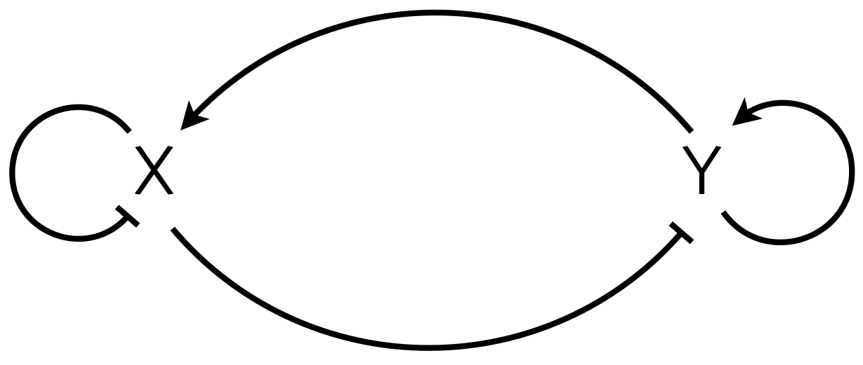
X and Y are coupled delay oscillators. X oscillates because of delayed repression, which we have been studying. Y oscillates via its X-mediated self-repression. Finally, the autoactivation of Y has bistability, a high and a low state as we saw in our early lessons. Due to the bistability, the toggle tends to push the oscillator to extremes, stabilizing the limit cycle. You may model this as a simple delay oscillator in your homework. Stricker and coworkers instead posited a multistep molecular mechanism to give oscillations. After their modeling confirmed oscillatory expression, they proceeded to design and build robust circuits using this architecture, as demonstrated from the movie from the paper below.