13. Stochastic differentiation
(c) 2019 Justin Bois and Michael Elowitz. With the exception of pasted graphics, where the source is noted, this work is licensed under a Creative Commons Attribution License CC-BY 4.0. All code contained herein is licensed under an MIT license.
This document was prepared at Caltech with financial support from the Donna and Benjamin M. Rosen Bioengineering Center.

This lesson was generated from a Jupyter notebook. Click the links below for other versions of this lesson.
Design principles
- Fast positive feedback combined with slow negative feedback can combine to give excitable circuits.
Concepts
- Excitable circuits have a unique, globally attracting rest state and a large stimulus can send the system on a long excursion before it returns to the resting state.
Techniques
- Plots of phase portraits.
import numpy as np
import scipy.integrate
import numba

import biocircuits

import bokeh.io
import bokeh.plotting

bokeh.io.output_notebook()
Noise: A bug or feature?
In the past two lessons, we have studied noise, how it comes about, how to quantify it, and how to take it into account when we study the dynamics of biological circuits. Noise is certainly a part of biological circuits, but is noise a bug for a feature?
We often regard noise as an unavoidable nuisance in biological life, especially at the scale of an individual cell. Perhaps we have this view because noise, by design, is generally absent from electronic circuits, which operate essentially deterministically. But perhaps noise could provide functional enabling capabilities for cells and organisms. If so, we can think about what these capabilities may be, and further how they are implemented by the circuits.
Excitability as a property of a dynamical system
We have seen seen several properties of dynamical systems enable cellular capabilities. Examples are in the table below.
| Dynamical system property | Cellular capability |
|---|---|
| Monostable fixed point | Remain in a constant state |
| Bistability | Exist in multiple epigenetically stable states (e.g., toggle switch) |
| Limit cycles | Ability to maintain oscillations (e.g., repressilator) |
In this lesson, we will discuss how another property of dynamical systems, that of excitability, may be used to enable probabilistic and transient differentiation events. We will discuss this in the context of cellular competence, which we discuss in the next section.
Excitability is tricky to define. Borrowing from Strogatz (in Nonlinear Dynamics and Chaos) an excitable system has two key properties:
- It has a unique, globally attracting rest state;
- A large enough stimulus can send the system on a long excursion before it returns to the resting state.
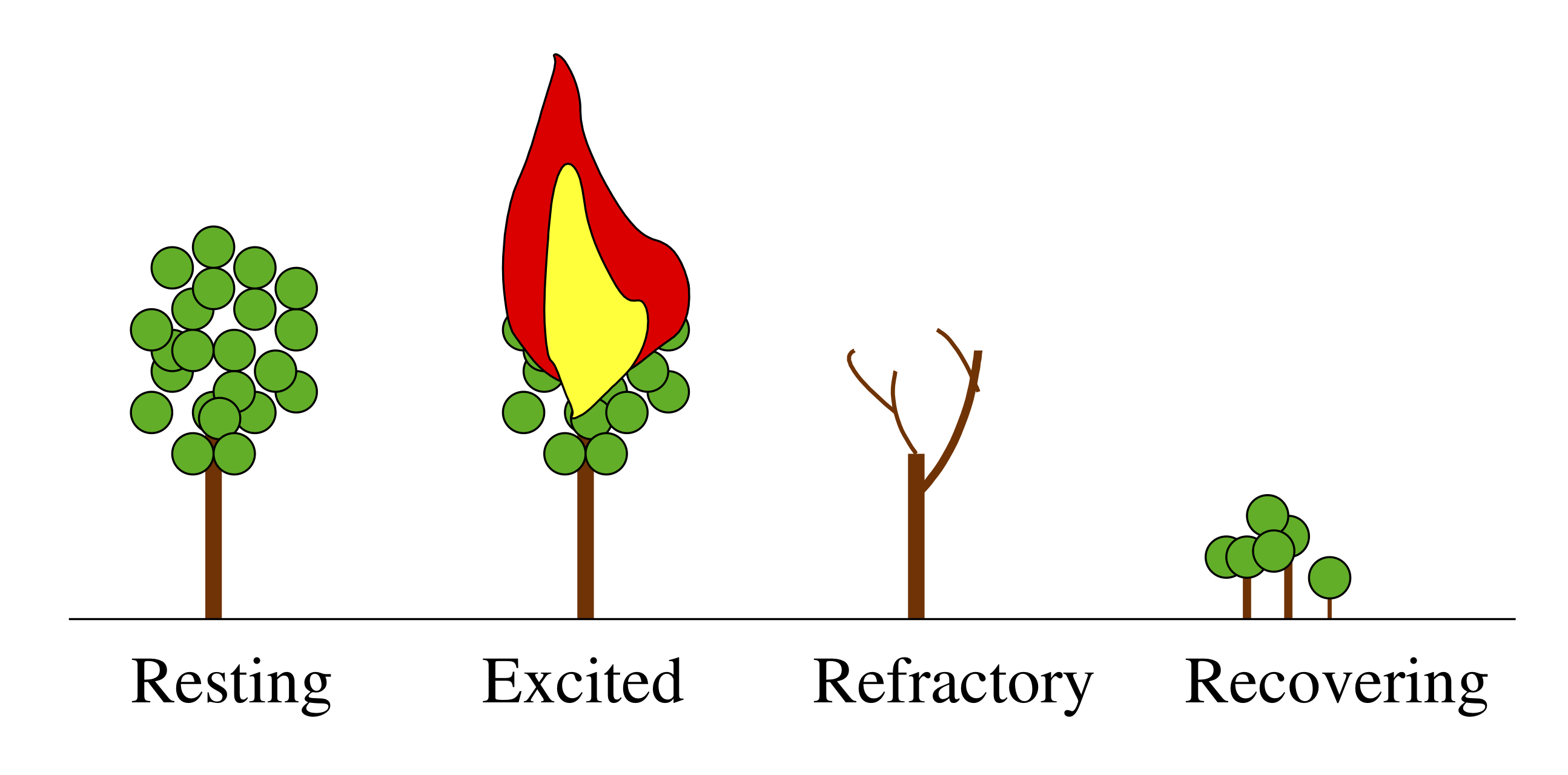
A forest is a classic example of an excitable system. Its resting state consists of many trees peacefully photosynthesizing and providing shade for hikers. Occasionally, though, an errant lightning strike or a careless camper can perturb the system on a large excursion wherein the forest burns, recovers, and then grows back again.
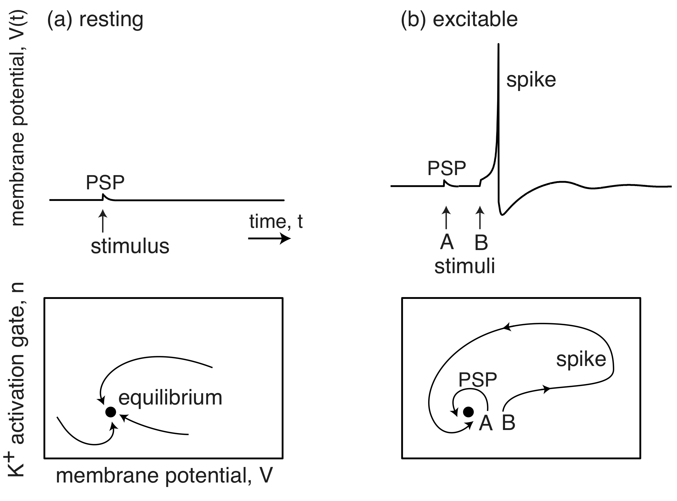
The membrane potentials of neurons are also excitable systems. When resting, they sit at their postsynaptic potential (PSP) and a stimulus results in them relaxing immediately back to their PSP. However, when they are excitable, a stimulus and lead to a big excursion wherein the membrane potential grows far beyond the PSP, before returning back to the PSP. This excursion is called a spike.
Importantly, stochastic fluctuations can be the source of the perturbation that pushes an excitable circuit off on one of its excursions.
Cellular competence
When stressed, bacterial species, like Bacillus subtilis, have several responses.
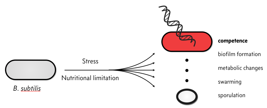
In particular, they can become competent, which means that they can take up environmental DNA. There is plenty of speculation as to the evolutionary advantage of competence, but we will not discuss that here. Rather, we will discuss the circuit governing how B. subtilis cells switch between a non-competent state, called a vegetative state to a competent one.
The response of individual cells to a stress is heterogeneous; some cells sporulate, some remain vegetative, some become competent, some die, etc.
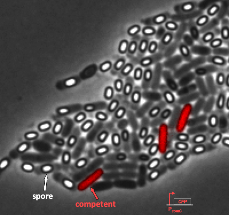
We can see this even more clearly in time lapse video. As we will discuss in a moment when we introduce the circuit responsible for competence, competent cells show up as pink/purple in the movie below.
In the video, it is evident that competence is both probabilistic (only a few cells become competent) and transient (competence is a temporary condition). These are hallmarks of excitability, and we will not examine the genetic circuit responsible for this excitability. In particular, we see to address the following questions.
- How do cells enter and exit competence?
- How do cells regulate the frequency and duration of competence?
- Can these properties be tuned?
- Is noise necessary to induce competence?
The B. subtilis competence circuit
The genetic circuit responsible for competence is connected to receptors responsible for sensing the environment and other circuits within the cell. The result can be a bit complicated, as shown in the figure below.
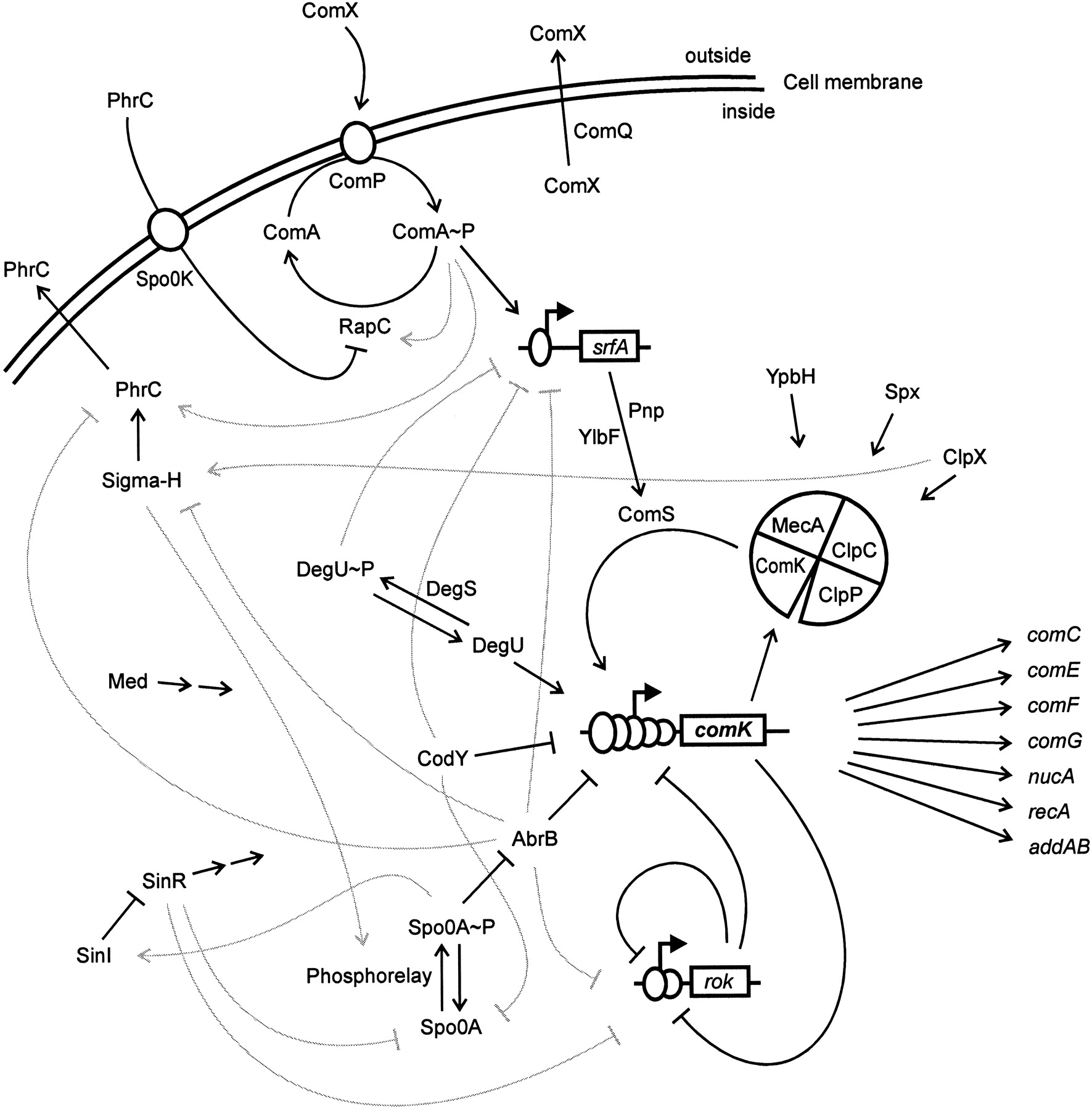
At the core of the circuit is ComK, which is necessary and sufficient for differentiation into competence. A simplified circuit, focusing on this ComK core, taken from [Süel, et al., *Nature*, 2006](https://doi.org/10.1038/nature04588), is shown below.
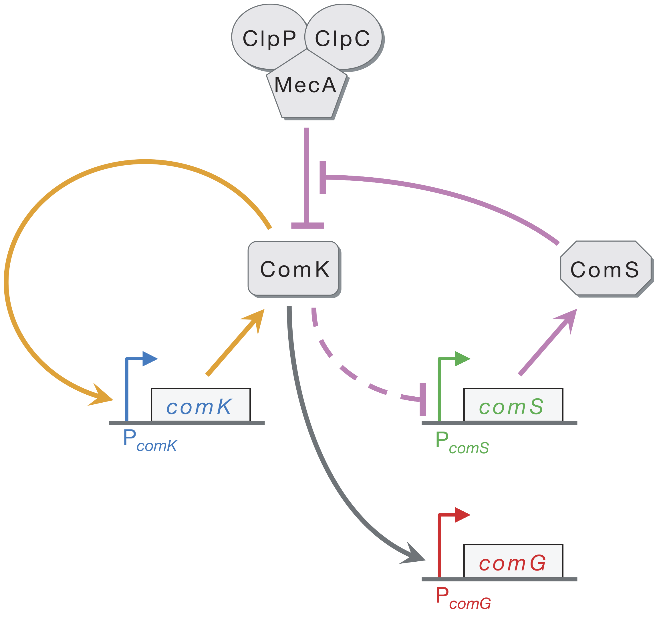
ComK activates its own transcription in a positive feedback loop (orange). ComK indirectly represses ComS (as marked by the dashed line). ComK is also degraded by the MecA–ClpP–ClpC complex (which we will call MecA for short), but so is ComS. This competition for degradation by MecA effectively means that ComS inhibits degradation of ComK by MecA. Finally, ComG is one of the genes activated by ComK that result in competence.
Süel and coworkers inserted pairwise combinations of the promoters for comK, comG and comS expression YFP and CFP in B. subtilis to monitor the levels of those genes. This is why the competent cells appeard purple in the movie above; both ComK (blue channel) and ComG (red channel) are active in competent cells.
We can look at the circuit to reason how it might be excitable. Imagine there is a transient excitement of ComK levels. This excitement is amplified by positive feedback (the orange arrows), leading to more production of ComK. There is enough ComS around to keep MecA from degrading the ComK molecules that are made due to the positive feedback. On a longer time scale, however, production of ComS gets inhibited, which results in the MecA complex starting to degrade ComK instead of ComS. This brings ComK back to its pre-excitedment level. In this sense, ComS serves to help initiate competence by reducing degradation of ComK, but also serves to bring the exit of competence when it is repressed by the excessive ComK.
This leads to a design principle. Fast positive feedback combined with slow negative feedback can combine to give excitable circuits.
In what follows, we will explore this competence circuit in more detail to get a quantitative understanding of how it works.
A model for the ComK circuit
To model the ComK circuit, we will follow the logic of Süel, et al. (Science, 2007). The MecA complex degrades ComK and ComS. ComS serves to inhibit this degradation by tying up the MecA complex in degrading itself. That is, there are two competing reactions: degradation of ComK and degradation of ComS. We take both of these reaction to have Michaelis-Menten kinetics, giving the reaction schemes
\begin{align} &\text{MecA} + \text{ComK} \stackrel{\gamma_{\pm a}}{\rightleftharpoons} \text{MecA-ComK} \stackrel{\gamma_1}{\rightarrow} \text{MecA} \\[1em] &\text{MecA} + \text{ComS} \stackrel{\gamma_{\pm b}}{\rightleftharpoons} \text{MecA-ComS} \stackrel{\gamma_2}{\rightarrow} \text{MecA}. \end{align}ComK is also known to indirectly inhibit expression of ComS, denoted by the dashed arrow. We take this to be described by a Hill function. Finally, ComK has a basal expression level. We can therefore write the dynamical equations for ComK and the MecA-ComK complex as
\begin{align} \frac{\mathrm{d}K}{\mathrm{d}t}&= \alpha_k + \beta_k\,\frac{K^n}{k_k^n + K^n} - \gamma_a M_f K + \gamma_{-a}M_K - \gamma_k K,\\[1em] \frac{\mathrm{d}M_K}{\mathrm{d}t} &= -(\gamma_{-a} + \gamma_1)M_K + \gamma_aM_f K, \end{align}where we have denoted the concentration of MecA-ComK as $M_K$ and of free MecA as $M_f$. We have also assumed that ComK undergoes non-catalyzed degradation, characterized by degradation rate $\gamma_k$.
We write the influence of ComK on ComS expression as a repressive Hill function. With our assumption of Michaelis-Menten kinetics on ComS degradation by MecA, we can now write the dynamical equations for ComS and the ComS-MecA complex.
\begin{align} \frac{\mathrm{d}S}{\mathrm{d}t}&= \frac{\beta_s}{1 + (K/k_s)^p} - \gamma_b M_f S + \gamma_{-b}M_S - \gamma_s S,\\[1em] \frac{\mathrm{d}M_S}{\mathrm{d}t} &= -(\gamma_{-b} + \gamma_2)M_S + \gamma_b M_f S. \end{align}Now, if we assume that the conversion of the MecA-Com complexes are very fast ($\gamma_1$ and $\gamma_2$ are large), we can make a pseudo-steady state approximation such that $\mathrm{d}M_K/\mathrm{d}t \approx \mathrm{d}M_S/\mathrm{d}t \approx 0$. Finally, if we assume that the total amount of MecA complex is conserved, i.e., $M_f + M_K + M_S = M_\mathrm{total} \approx \text{constant}$, we can simply our expressions. Specifically, we now have
\begin{align} \frac{\mathrm{d}K}{\mathrm{d}t}&= \alpha_k + \beta_k\,\frac{K^n}{k_k^n + K^n} -\gamma_1M_K - \gamma_k K,\\[1em] \frac{\mathrm{d}S}{\mathrm{d}t}&= \alpha_s + \frac{\beta_s}{1 + (K/k_s)^p} - \gamma_2 M_S - \gamma_s S. \end{align}We can get expressions for $M_K$ and $M_S$ in terms of $M_\mathrm{total}$, $K$, and $S$ by using the relations following our two assumptions,
\begin{align} -(\gamma_{-a} + \gamma_1)M_K + \gamma_a(M_\mathrm{total} - M_K - M_S) K &= 0,\\[1em] -(\gamma_{-b} + \gamma_2)M_S + \gamma_b(M_\mathrm{total} - M_K - M_S) S &= 0. \end{align}We can write these in a more convenient form to eliminate $M_K$ and $M_S$.
\begin{align} (\gamma_{-a} + \gamma_1 + \gamma_a K)M_K + \gamma_a K M_S &= \gamma_a M_\mathrm{total} K \\[1em] \gamma_b S M_K + (\gamma_{-b} + \gamma_2 + \gamma_b S)M_S &= \gamma_b M_\mathrm{total} S. \end{align}Solving this system of linear equations for $M_K$ and $M_S$ yields
\begin{align} M_K &= M_\mathrm{total}\,\frac{K/\Gamma_k}{1 + K/\Gamma_k + S/\Gamma_s}, \\[1em] M_S &= M_\mathrm{total}\,\frac{S/\Gamma_s}{1 + K/\Gamma_k + S/\Gamma_s}, \end{align}where $\Gamma_k \equiv (\gamma_{-a} + \gamma_1)/\gamma_a$ and $\Gamma_k \equiv (\gamma_{-b} + \gamma_2)/\gamma_b$. Inserting these expressions back into our ODEs for the $K$ and $S$ dynamics and defining $\delta_k\equiv \gamma_1 M_\mathrm{total}/\Gamma_k$ and $\delta_s \equiv\gamma_2 M_\mathrm{total}/\Gamma_s$ for notational convenience yields
\begin{align} \frac{\mathrm{d}K}{\mathrm{d}t}&= \alpha_k + \beta_k\,\frac{K^n}{k_k^n + K^n} - \frac{\delta_k K}{1 + K/\Gamma_k + S/\Gamma_s} - \gamma_k K\\[1em] \frac{\mathrm{d}S}{\mathrm{d}t}&= \alpha_s + \frac{\beta_s}{1 + (K/k_s)^p} - \frac{\delta_s S}{1 + K/\Gamma_k + S/\Gamma_s} - \gamma_s S. \end{align}We will nondimensinalize time by the rate of ComK degradation by the MecA complex, $\delta_k$. The parameters $\Gamma_k$ and $\Gamma_s$ are natural choices for nondimensionalizing $K$ and $S$. The resulting dimensionless equations are
\begin{align} \frac{\mathrm{d}k}{\mathrm{d}t}&= a_k + \frac{b_k\,(k/\kappa_k)^n}{1 + (k/\kappa_k)^n} - \frac{k}{1 + k + s} - \gamma_k k, \\[1em] \frac{\mathrm{d}s}{\mathrm{d}t}&= a_s + \frac{b_s}{1 + (k/\kappa_s)^p} - \frac{s}{1 + k + s} - \gamma_s s. \end{align}It is left to the reader to work out the relationships between the dimensionless and dimensional parameters.
Analysis of the dynamical system
Now that we have our dynamic system set up, we can begin analysis. We will start by defining parameters for the system, using the parameters specified in the Süel, et al. paper. For convenience, we will store the parameters in a container.
class CompetenceParams(object):
    """
    Container for parameters for B. subtilis competence circuit.
    """
    def __init__(self, **kwargs):
        # Dimensionless parameters
        self.a_k = 0.00035
        self.a_s = 0.0
        self.b_k = 0.3
        self.b_s = 3.0
        self.kappa_k = 0.2
        self.kappa_s = 1/30
        self.gamma_k = 0.1
        self.gamma_s = 0.1
        self.n = 2
        self.p = 5

        # Put in params that were specified in input
        for entry in kwargs:
            setattr(self, entry, kwargs[entry])
With the parameters in hand, we can define the time derivatives for the dimensionless ComK and ComS concentrations.
def dk_dt(k, s, p):
    """p is a CompetenceParams instance"""
    return (p.a_k + p.b_k * k**p.n / (p.kappa_k**p.n + k**p.n)
                    - k / (1 + k + s) - p.gamma_k*k)

def ds_dt(k, s, p):
    return p.a_s + p.b_s / (1 + (k / p.kappa_s)**p.p) - s / (1 + k + s) - p.gamma_s*s
We have seen that plotting the nullclines is a useful exercise, as this exposes the fixed points. This this system, the nullclines are most easily represented in for form $s(k)$, that is, $s$ as a function of $k$. These are easily derived by setting $\mathrm{d}k/\mathrm{d}t$ and $\mathrm{d}s/\mathrm{d}t$ equal to zero.
\begin{align} &\frac{\mathrm{d}k}{\mathrm{d}t} = 0 \;\Rightarrow s\; = \frac{k}{a_k - \gamma_k k + b_k k^n / (\kappa_k^n + k^n)} - k - 1. \end{align}The nullcline given by $\mathrm{d}s/\mathrm{d}t = 0$ is the positive root of the quadratic polynomial equation $as^2 + b s + c = 0$ with
\begin{align} a &= \gamma_s,\\[1em] b &= 1 + \gamma_s(1+k) - A,\\[1em] c &= -A(1+k), \end{align}with
\begin{align} A = a_s + \frac{b_s}{(1 + (k/\kappa_s)^p}. \end{align}We can code these up.
def k_nullcline(k, p):
    abk = p.a_k + p.b_k * k**p.n / (p.kappa_k**p.n + k**p.n) - p.gamma_k * k
    return k / abk - k - 1

def s_nullcline(k, p):
    A = p.a_s + p.b_s / (1 + (k / p.kappa_s)**p.p)
    a = p.gamma_s
    b = 1 - A + p.gamma_s * (1 + k)
    c = -A * (1 + k)

    return -2*c / (b + np.sqrt(b**2 - 4*a*c))
We will being our graphical analysis by plotting the nullclines, as we have done in past lessons. Knowing what our demands will be in a moment when plotting the phase portrait, we will write a function to plot the nullclines where the $k$ and $s$ axes are on a logarithmic scale and also on a linear scale.
def plot_nullclines(k_range, log=True, p=None, **kwargs):
    """
    Compute and plot the nullclines.
    """
    if p is None:
        p = bokeh.plotting.figure(plot_width=350, plot_height=260,
                                  x_axis_label='log₁₀ k',
                                  y_axis_label='log₁₀ s',
                                  **kwargs)

    if log:
        k = np.logspace(np.log10(k_range[0]), np.log10(k_range[1]), 200)
        s_nck = k_nullcline(k, params)
        s_ncs = s_nullcline(k, params)
        p.line(np.log10(k), np.log10(s_nck), color='#ff7f0e', line_width=3)
        p.line(np.log10(k), np.log10(s_ncs), color='#9467bd', line_width=3)
    else:
        k = np.linspace(k_range[0], k_range[1], 200)
        s_nck = k_nullcline(k, params)
        s_ncs = s_nullcline(k, params)
        p.line(k, s_nck, color='#ff7f0e')
        p.line(k, s_ncs, color='#9467bd')

    return p
We can now use this function to make the plot. We will use the parameter values from the Süel, et al. paper and make the plot with $k$ and $s$ on a logarithmic scale. Note that we are labeling our axes as "log₁₀ [ComK]" instead of choosing x_axis_type = 'log' as a keyword argument when building the figure. Our reason for doing this will become clear when we add a phase portrait to the plot.
params = CompetenceParams()
k_range = np.array([1e-3, 2])
s_range = np.array([1e-3, 5000])

p = plot_nullclines(k_range, log=True, y_range=np.log10(s_range))
bokeh.io.show(p)
The nullclines have three crossings, implying three fixed points. To investigate the behavior near the fixed point, and indeed away from them as well, we can plot the phase portrait. A phase portrait is a plot displaying possible trajectories of a dynamical system in phase space, in this case on the $k$-$s$ plane. Let's generate a phase portrait using the biocircuits package (with the nullclines overlaid) to look at one, and then we will revisit how it is generated.
# Make the plot
p = biocircuits.phase_portrait(dk_dt, ds_dt, k_range, s_range,
                               (params,), (params,), log=True,
                               x_axis_label='log₁₀ k',
                               y_axis_label='log₁₀ s',
                               plot_width=350)
p = plot_nullclines(k_range, log=True, p=p)

bokeh.io.show(p)
The phase portrait is intuitive. The streamlines depict how the system evolves with time. Coming from the top (lots of ComS is around), if $k$ is small (there is not much ComK around), the system tends toward the leftmost fixed point. If $k$ is larger, though, the system makes an excursion to large $k$ values, and then drops to large $k$/low $s$, before returning back to the leftmost fixed point. This is indeed the hallmark of an excitable system. It takes a large excursion in phase space before returning to a stable fixed point.
To better understand the dynamics close to the fixed points, we can take a closer look.
k_range = [0.0025, 0.0030]
s_range = [15, 30]

p = biocircuits.phase_portrait(dk_dt, ds_dt, k_range, s_range,
                               (params,), (params,), log=True,
                               x_axis_label='log₁₀ k',
                               y_axis_label='log₁₀ s',
                               plot_width=350)
p = plot_nullclines(k_range, log=True, p=p)

bokeh.io.show(p)
This is a stable fixed point, with the system flowing into it from all directions (when $k$ and $s$ are close to the fixed point). Let's now look at the fixed point for the next largest $k$.
k_range = [0.014, 0.02]
s_range = [10, 30]

p = biocircuits.phase_portrait(dk_dt, ds_dt, k_range, s_range,
                               (params,), (params,), log=True,
                               x_axis_label='log₁₀ k',
                               y_axis_label='log₁₀ s',
                               plot_width=350)
p = plot_nullclines(k_range, log=True, p=p)

bokeh.io.show(p)
We can see from the flow lines that this is an unstable fixed point, a saddle. We could perform linear stability analysis on this fixed point, and we would find a positive trace and a negative determinant of the linear stability matrix. This means that the system comes toward the fixed point from one direction, but is pushed away along the other.
Finally, let's look at the last fixed point, for largest $k$.
k_range = [0.02, 0.05]
s_range = [1, 15]

p = biocircuits.phase_portrait(dk_dt, ds_dt, k_range, s_range,
                               (params,), (params,), log=True,
                               x_axis_label='log₁₀ k',
                               y_axis_label='log₁₀ s',
                               plot_width=350)
p = plot_nullclines(k_range, log=True, p=p)

bokeh.io.show(p)
This fixed point is a spiral source. It is unstable and spirals the system away from it.
Numerical solution of dynamical equations
Now that we have a good picture of the dynamics, we can numerically solve the dynamical equations. Of course, the initial conditions are relevant here. We will start with no ComK or ComS (which is not at all relevant physiologically) and solve.
# Right-hand-side of ODEs
def rhs(ks, t, p):
    """
    Right-hand side of dynamical system.
    """
    k, s = ks
    return np.array([dk_dt(k, s, p), ds_dt(k, s, p)])

# Set up and solve
t = np.linspace(0, 200, 100)
ks_0 = np.array([0, 0])
ks = scipy.integrate.odeint(rhs, ks_0, t, args=(params,))
k, s = ks.transpose()
We will plot this in phase space, with the nullclines overlaid. The trajectory is in gray.
params = CompetenceParams()
k_range = np.array([1e-3, 2])
s_range = np.array([1e-3, 5000])

p = plot_nullclines(k_range, log=True, y_range=np.log10(s_range))
p.line(np.log10(k[1:]), np.log10(s[1:]), line_width=2, color='gray')

bokeh.io.show(p)
We see a rise to the fixed point. Now, let's say we had some fluctuation that kicked us up a bit off of the fixed point. We'll start with $s = 6$ and $k = 0.05$ and we'll color the trajectory in a blue color.
# Set up and solve
t = np.linspace(0, 200, 300)
ks_0 = np.array([1e-2, 1e3])
ks = scipy.integrate.odeint(rhs, ks_0, t, args=(params,))
k2, s2 = ks.transpose()

p.line(np.log10(k2), np.log10(s2), line_width=2, color='steelblue')

bokeh.io.show(p)
The system takes a much longer trajectory to get to the fixed point, taking the excursion we suspected it would from the phase portrait.
Stochastic simulation
As we have just seen, the system can take a transient journey into competence provided it is perturbed far enough away from the stable fixed point. This raises the question, is intrinsic noise enough to give the "kick" needed to make the excursion to compentence? To investigate this, we can perform a Gillespie simulation (SSA) to investigate the dynamics. To specify the master equation, we need the usual ingredients.
- A definition of the species present with variables representing their copy number.
- A definition of the unit moves that are allowed (the nonzero transition kernels).
- Updates to copy numbers for each move.
- The propensity for each move.
We can conveniently organize these in tables. First, the variables.
| index | description | variable |
|---|---|---|
| 0 | comK mRNA copy number | mk |
| 1 | ComK protein copy number | pk |
| 2 | comS mRNA copy number | ms |
| 3 | ComS protein copy number | ps |
| 4 | Free MecA complex copy number | af |
| 5 | MecA-ComK complex copy number | ak |
| 6 | MecA-ComS complex copy number | as_ |
With the species defined, we an write the move set with propensities.
| index | description | update | propensity |
|---|---|---|---|
| 0 | constitutive transcription of a comK mRNA | mk ⟶ mk + 1 |
k1 * P_comK_const |
| 1 | regulated transcription of a comK mRNA | mk ⟶ mk + 1 |
P_comK * f(k, k2, kappa_k, n) |
| 2 | translation of a ComK protein | pk ⟶ pk + 1 |
k3 * mk |
| 3 | constitutive transcription of a comS mRNA | ms ⟶ ms + 1 |
k4 * P_comS_const |
| 4 | regulated transcription of a comS mRNA | ms ⟶ ms + 1 |
P_comS * g(k, k5, kappa_s, p) |
| 5 | translation of a ComS protein | ps ⟶ ps + 1 |
k6 * ms |
| 6 | degradation of a comK mRNA | mk ⟶ mk - 1 |
k7 * mk |
| 7 | degradation of a comK protein | pk ⟶ pk - 1 |
k8 * pk |
| 8 | degradation of a comS mRNA | ms ⟶ ms - 1 |
k9 * ms |
| 9 | degradation of a comS protein | ps ⟶ ps - 1 |
k10 * ps |
| 10 | binding of MecA and ComK | af ⟶ af - 1, pk ⟶ pk - 1, ak ⟶ ak + 1 |
k11 * af * pk / omega |
| 11 | unbinding of MecA and ComK | af ⟶ af + 1, pk ⟶ pk + 1, ak ⟶ ak - 1 |
km11 * a_k |
| 12 | degradation ComK by MecA | af ⟶ af + 1, ak ⟶ ak - 1 |
k12 * ak |
| 13 | binding of MecA and ComS | af ⟶ af - 1, ps ⟶ ps - 1, as_ ⟶ as_ + 1 |
k13 * af * ps/\Omega |
| 14 | unbinding of MecA and ComS | af ⟶ af +1, ps ⟶ ps + 1, as_ ⟶ as_ - 1 |
km13 * as_ |
| 15 | degradation ComS by MecA | af ⟶ af + 1, as_ ⟶ as_ - 1 |
k14 * as_ |
In defining the propensities, we introduced parameters. We can define their values, again in accordance with the Süel, et al. paper.
| parameter | value | units |
|---|---|---|
P_comK_const |
1 | - |
P_comS_const |
1 | - |
P_comK |
1 | - |
P_comS |
1 | - |
omega |
1 | molecule/nM |
k1 |
0.00021875 | 1/sec |
k2 |
0.1875 | 1/sec |
k3 |
0.2 | 1/sec |
k4 |
0 | - |
k5 |
0.0015 | 1/sec |
k6 |
0.2 | 1/sec |
k7 |
0.005 | 1/sec |
k8 |
0.0001 | 1/sec |
k9 |
0.005 | 1/sec |
k10 |
0.0001 | 1/sec |
k11 |
2.02×10$^{-6}$ | 1/nM-sec |
km11 |
0.0005 | 1/sec |
k12 |
0.05 | 1/sec |
k13 |
4.5×10$^{-6}$ | 1/nM-sec |
km13 |
5×10$^{-5}$ | 1/nM-sec |
k14 |
4×10$^{-5}$ | 1/sec |
kappa_k |
5000 | nM |
kappa_s |
833 | nM |
n |
2 | - |
p |
5 | - |
Additionally, we take the total MecA complex copy number to be 500. That is, af+ak+as_ = 500.
We now have all the ingredients, so we can proceed to code up the simulation.
@numba.njit
def propensity(propensities, population, t,
               P_comK_const,
               P_comS_const,
               P_comK,
               P_comS,
               omega,
               k1,
               k2,
               k3,
               k4,
               k5,
               k6,
               k7,
               k8,
               k9,
               k10,
               k11,
               km11,
               k12,
               k13,
               km13,
               k14,
               kappa_k,
               kappa_s,
               n,
               p):
    mk, pk, ms, ps, af, ak, as_ = population

    f_num = (pk / kappa_k * omega)**n
    f = k2 * f_num / (1 + f_num)
    g = k5 / (1 + (pk / kappa_s * omega)**p)

    propensities[0] = k1 * P_comK_const
    propensities[1] = P_comK * f
    propensities[2] = k3 * mk
    propensities[3] = k4 * P_comS_const
    propensities[4] = P_comS * g
    propensities[5] = k6 * ms
    propensities[6] = k7 * mk
    propensities[7] = k8 * pk
    propensities[8] = k9 * ms
    propensities[9] = k10 * ps
    propensities[10] = k11 * af * pk / omega
    propensities[11] = km11 * ak
    propensities[12] = k12 * ak
    propensities[13] = k13 * af * ps / omega
    propensities[14] = km13 * as_
    propensities[15] = k14 * as_


update = np.array([
    # 0   1   2   3   4   5   6
    [ 1,  0,  0,  0,  0,  0,  0], # 0
    [ 1,  0,  0,  0,  0,  0,  0], # 1
    [ 0,  1,  0,  0,  0,  0,  0], # 2
    [ 0,  0,  1,  0,  0,  0,  0], # 3
    [ 0,  0,  1,  0,  0,  0,  0], # 4
    [ 0,  0,  0,  1,  0,  0,  0], # 5
    [-1,  0,  0,  0,  0,  0,  0], # 6
    [ 0, -1,  0,  0,  0,  0,  0], # 7
    [ 0,  0, -1,  0,  0,  0,  0], # 8
    [ 0,  0,  0, -1,  0,  0,  0], # 9
    [ 0, -1,  0,  0, -1,  1,  0], # 10
    [ 0,  1,  0,  0,  1, -1,  0], # 11
    [ 0,  0,  0,  0,  1, -1,  0], # 12
    [ 0,  0,  0, -1, -1,  0,  1], # 13
    [ 0,  0,  0,  1,  1,  0, -1], # 14
    [ 0,  0,  0,  0,  1,  0, -1]  # 15
    ], dtype=int)

# Parameter values
P_comK_const = 1
P_comS_const = 1
P_comK = 1
P_comS = 1
omega = 1
k1 = 0.00021875
k2 = 0.1875
k3 = 0.2
k4 = 0.0
k5 = 0.0015
k6 = 0.2
k7 = 0.005
k8 = 0.0001
k9 = 0.005
k10 = 0.0001
k11 = 2.02e-6
km11 = 0.0005
k12 = 0.05
k13 = 4.5e-6
km13 = 5e-5
k14 = 4e-5
kappa_k = 5000.0
kappa_s = 833.0
n = 2
p = 5

args = (P_comK_const,
        P_comS_const,
        P_comK,
        P_comS,
        omega,
        k1,
        k2,
        k3,
        k4,
        k5,
        k6,
        k7,
        k8,
        k9,
        k10,
        k11,
        km11,
        k12,
        k13,
        km13,
        k14,
        kappa_k,
        kappa_s,
        n,
        p)

population_0 = np.array([10, 100, 10, 400, 500, 0, 0], dtype=int)

time_points = np.linspace(0, 4000000, 4001)
All of the required arguments are set, so let's now run a trajectory. When we plot the trajectory, we will show it along with the phase protrait (with counts adjusted to the same dimensionless concentration units).
# Perform the Gillespie simulation
pop = biocircuits.gillespie_ssa(propensity, update, population_0, time_points, args=args)

k = pop[0, :, 1] / omega * k11 / (km11 + k12)
s = pop[0, :, 3] / omega * k13 / (km13 + k14)

# Make plot
k_range = np.array([1e-4, 2])

# Make the plot
p = biocircuits.phase_portrait(dk_dt, ds_dt, k_range, s_range,
                               (params,), (params,), log=True,
                               x_axis_label='log₁₀ k',
                               y_axis_label='log₁₀ s',
                               plot_width=350)
p = plot_nullclines(k_range, log=True, p=p)
p.line(np.log10(k), np.log10(s), level='underlay', color='gray')

bokeh.io.show(p)
The warning message and the broken line of the trajectory are due to some counts going identically to zero, which cannot be displayed on a log scale. In looking at the trajectory, we see that the system stays near the stable fixed point, but fluctuations due solely to small copy numbers are enough to occasionally send the system on a trajectory toward competence and then back to the stable fixed point.