14. Cellular 'bet-hedging'
(c) 2019 Justin Bois and Michael Elowitz. With the exception of pasted graphics, where the source is noted, this work is licensed under a Creative Commons Attribution License CC-BY 4.0. All code contained herein is licensed under an MIT license.
This document was prepared at Caltech with financial support from the Donna and Benjamin M. Rosen Bioengineering Center.

This lesson was generated from a Jupyter notebook. Click the links below for other versions of this lesson.
Design principle
- When environmental conditions fluctuate unpredictably, bet-hedging through spontaneous, probabilistic cellular state-switching (differentiation) can outperform adaptive response strategies.
Concepts
- Kelly betting
- Antibiotic persistence
Techniques
- Optimal betting strategies
- Single cell movies
Survival in an uncertain world requires adaptability and anticipation, the complementary abilities to respond to and prepare for change.
— Jeffrey N. Carey and Mark Goulian, "A bacterial signaling system regulates noise to enable bet hedging," Current Genetics, 2019.
Bacteria are like money
We begin with a very loose analogy between money and bacteria.
One can try to optimize one's financial interests through a portfolio of investments. If you knew exactly which stocks were going to increase in value, by how much, and when, then you could put all your money in the fastest growing stock. However, in real life, there is great uncertainty. How much one invests, and how one distributes the total investment across specific stocks or funds will depend depend on some estimate of the probabilities that those stocks will increase or decrease in value.
Bacteria face a similar challenge. Individual cells can exist in a variety of physiological states, better or worse adapted to various potential future environments. Put a bacterial cell in the "right" state to anticipate the environment it will face, and it could proliferate more rapidly than its cousins. By contrast, put it in the wrong state and it may simply not survive the coming environmental change at all.
Just as future stock prices are hard to predict, so too are environmental fluctuations: temperature, salt, toxins, antibiotics, and attacking immune cells may or may not appear at any time.
In the financial context, a common strategy is to spread your investments across multiple stocks. If any one fails, you do not lose everything. (Although broad-based correlations across the market can limit the independence of individual stocks). This is a form of bet hedging.
In the case of cells, different subsets of a cell population can differentiate into various alternative states, each adapted to anticipate different possible future environmental conditions. One way to think of this is as a hedge produced by the shared genome of that (clonal) cell population, which spreads its bets, in the form of individual cells, across multiple physiological states.
An ideal cell for an uncertain world
Today, we seek to gain some insight into how bacteria can and do "bet" or "gamble." We imagine that we are designing a bacterial stress response system for a custom bacterium. Our goal is to maximize the survival and proliferation of the bug.
We can provide the cell with an array of sensors, information processing circuits, and responses. We also have the option, if we want, to incorporate a "random number generator" that operates independently in each individual cell. What kinds of benefits can one obtain using the random number generator that one could not obtain without it?
What is our random number generator? Noise! We have seen that gene expression occurs through intrinsically stochastic bursts of protein production, making the cell a "noisy machine." We further saw, through the example of bacterial competence, that this noise, when considered in the context of a regulatory circuit, enables cells to implement probabilistic strategies, by controlling the fraction of cells in the population that are in one state or another. The probabilities with which cells do one thing or another can, in general, depend on the environment, or even on its history.
This is fundamentally a gambling, or betting, question. And so, to begin, we will go through some classic results in the theory of optimal betting originally developed by John Kelly in 1956, following an excellent and highly recommended lecture from Thomas Ferguson at UCLA.
First, we will discuss the general concept of proportional gambling, or "Kelly betting."
Next, we will discuss a simple artificial example based on stochastic switching between two cellular states and two environments to see how to optimize growth. We will then extend this discussion to systems with multiple states and multiple corresponding environments, and if and when a purely probabilistic strategy can outperform one based on direct sensing of the environment.
Finally, we will highlight the particular phenomenon of antibiotic persistence, which presents a biomedical important example in which bacterial bet-hedging plays out.
A simple betting game
Following Ferguson, we start with the simplest betting game one can imagine: Each day you get to make a bet, and the odds of winning are always the same. Even better, unlike Vegas, the odds are actually in your favor, with your probability of winning, $p$, better than even: $p>0.5$.
All you have to decide is how much you want to bet each day. $b_k$ denotes the amount of your $k$th bet. It could range from 0 to your total fortune before the bet, denoted $X_{k-1}$. That is $0\le b_k \le X_{k-1}$.
If you win or lose the bet, you gain or lose $b_k$ dollars, respectively.
\begin{align} X_k = \begin{cases} X_{k-1} + b_k & \textrm{ with probability } p \\[1em] X_{k-1} - b_k & \textrm{ with probability } 1-p \end{cases} \end{align}"I'm ruined!"
How much should you bet each day?
Each day, because $p>1$, the bet that will maximize the "expectation value" of your wealth would be to bet everything, $b_k=X_{k-1}$.
If you won every single bet, your wealth would increase, after $k$ bets by a factor of $2^k$. However, the probability of winning $k$ bets in a row, $p^k$, is low even when $p$ is high. For instance, with $p=0.8$, you have less than only about 1.5% chance of surviving 20 rounds. This is the phenomenon of gambler's ruin.
Proportional betting
Since the odds are in your favor here, shouldn't there be a better strategy?
One obvious possibility is proportional betting. In this scheme, you set the size of your bet to be proportional to the amount of money you have: $b_k = f X_{k-1}$, where $0<f<1$ denotes the fraction of your wealth you bet on each round. Even if you lose, you are not wiped out completely. You still live to play another day.
What is the best value of $f$ to use in this scheme? Ideally, you would choose the value that maximizes the rate of increase of your wealth so you can reach your own personal comfort level as fast as possible and find something more meaningful to do with your time.
Let's consider one particular "run" of $n$ bets, in which you won $Z_n$ times and lost $n-Z_n$ times. After this run, your wealth has now changed from $X_0$ to
\begin{align} X_n = X_0 (1+f)^{Z_n}(1-f)^{n-Z_n}. \end{align}Of course, each run will be different depending on $Z_n$ and the distribution of possible $Z_n$'s is Binomial; $Z_n \sim \text{Binom}(n,p)$. We can express expected fold change in wealth.
\begin{align} \frac{\langle Z_n\rangle}{Z_0} = \langle (1+f)^{Z_n}(1-f)^{n-Z_n}\rangle, \end{align}which is in general difficult to calculate analytically. (We will do so by sampling out of the distribution of $Z_n$ momentarily.) We can, however, compute the expected logarithm of the fold change in wealth.
\begin{align} \left\langle \ln \frac{Z_n }{Z_0}\right \rangle &= \left\langle Z_n \ln (1+f) + (n - Z_n)\ln (1-f) \right\rangle \\[1em] &= n\ln (1-f) + \langle Z_n \rangle \, [\ln (1+f) - \ln (1-f)] \\[1em] &= n\left[p \ln (1+f) + (1-p) \ln (1-f)\right], \end{align}where in the last line we have used the fact that $Z_n$ is Binomially distributed, so $\langle Z_n \rangle = np$. We thus expect an exponential growth in wealth,
\begin{align} \mathrm{e}^{\langle \ln X_n\rangle} = X_0\,\mathrm{e}^{r n}, \end{align}where the growth rate is
\begin{align} r = p \ln (1+f) + (1-p) \ln (1-f). \end{align}This expression may remind you of Shannon's information—in fact, Kelly's 1956 article explores this connection and extends this analysis to many other interesting examples and connections.
Now we can answer the critical question: what is the optimal bet, $f$? To do so, just solve $ \frac{\mathrm{d}r}{\mathrm{d} f}=0$ to find the $f$ that maximizes the growth rate. The result is
\begin{align} f_{opt} = \begin{cases} 2p - 1 & p > 1/2,\\[1em] 0 & p \le 1/2. \end{cases} \end{align}For example, with a modest advantage like $p=0.55$, you would bet 10% each time. With a larger advantage like $p=0.9$, you could bet 80%.
A few interesting points about this result:
What if the odds are unfavorable? If $p<1/2$, you are better off (of course) not betting. Just go home.
This rule can be interpreted as maximizing the expectation value for the logarithm of total wealth.
This result can be generalized to the case where the probabilities change with time. In that case, each round one just replaces $p$ with $p_k$.
In his conclusion, Kelly writes (in dated language about the gambler's wife):
The gambler introduced here follows an essentially different criterion from the classical gambler. At every bet he maximizes the expected value of the logarithm of his capital. The reason has nothing to do with the value function which he attached to his money, but merely with the fact that it is the logarithm which is additive in repeated bets and to which the law of large numbers applies. Suppose the situation were different; for example, suppose the gambler's wife allowed him to bet one dollar each week but not to reinvest his winnings. He should then maximize his expectation (expected value of capital) on each bet. He would bet all his available capital (one dollar) on the event yielding the highest expectation. With probability one he would get ahead of anyone dividing his money differently.
See Tom Ferguson's lecture for other interesting extensions and applications.
Simulating Kelly betting
We worked out the expectation value of the logarithm of wealth. We might also be interested in learning about how individual outcomes of Kelly betting might play out and to gather information about the distribution of outcomes. To that end, we can simulate Kelly betting games. We do so below, starting with $X_0 = 1$ and betting 100 rounds, with $p = 0.6$, giving an optimal betting strategy of $f = 2p-1 = 0.2$.
Each series of bets is shown in a blue line, with the computed and theoretical expectation values shown. On average, the wealth grows, but we do occasionally lose.
It is also interesting to look at the distribution of outcomes: What is the distribution of outcomes after 100 rounds of betting? We can look at the ECDF of the betting outcomes.
We lose about 12% of the time, but we can still win big (the riches axis is on a logarithmic scale)!
Alternative bacterial strategies: sense and respond or stochastically switch?
What does this calculation have to do with bacteria?
Here we ask how a population of cells can survive and even thrive in unpredictable environments. Just as we ask how we can grow our financial portfolio and avoid ruin, so too we can ask how a clonal population of cells, implementing identical, but probabilistic, programs, can maximize their total growth rate and avoid elimination.
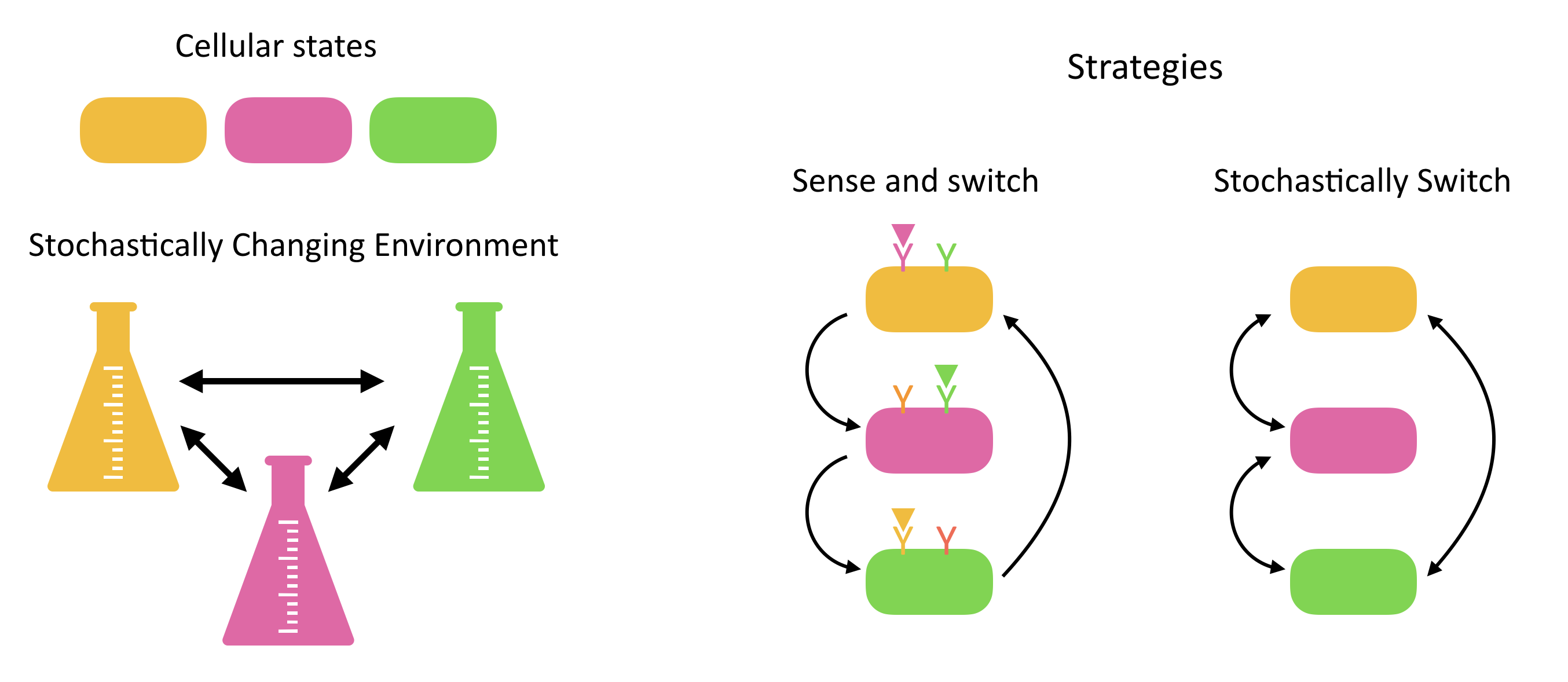
Responsive switching. At first glance, the most straightforward solution is to deterministically sense the current and environment and adjust expression of proteins to put cells into its best adapted state. However, this requires that cells express specific sensors for a broad variety of conditions that they may not encounter most of the time.
Stochastic switching. An alternative way to adapt is not to sense at all, but rather to just switch stochastically between different states, "hoping" that the cost from having cells in less adaptive states some of the time will be outweighed by the reduced cost of constantly sensing a broad variety of different inputs. In fact, many natural systems appear to implement such stochastic state-switching strategies.
Of course, both strategies could be used together in any particular system.
There are now many well-known examples in which cells appear to use stochastic switching strategies:
- Salmonella uses "phase variation" to switch between different epitopes and thereby evade detection by the immune system.
- Bacterial cells stochastically enter and exit "persistent" states that are less susceptible to antibiotics.
- Sporulation and competence appear to initiate stochastically in individual cells of Bacillus subtilis.
- Antibiotic peristence -- which we will discuss momentarily.
Optimizing stochastic switching for environmental variation:
We first ignore the sensing strategy and focus on a purely stochastic strategy.
Thattai and van Oudenaarden, (Genetics, 2003) considered a minimal case in which cells can switch between two distinct states, each optimized for growth in one of two possible environments. They assumed that both the environment and the cells switch stochastically between their respective states. However, the cell is assumed not to directly sense the environment it is in.
In a subsequent paper, Acar et al, (Nature Genetics, 2008), the same group constructed an experimental realization of these conditions in yeast.
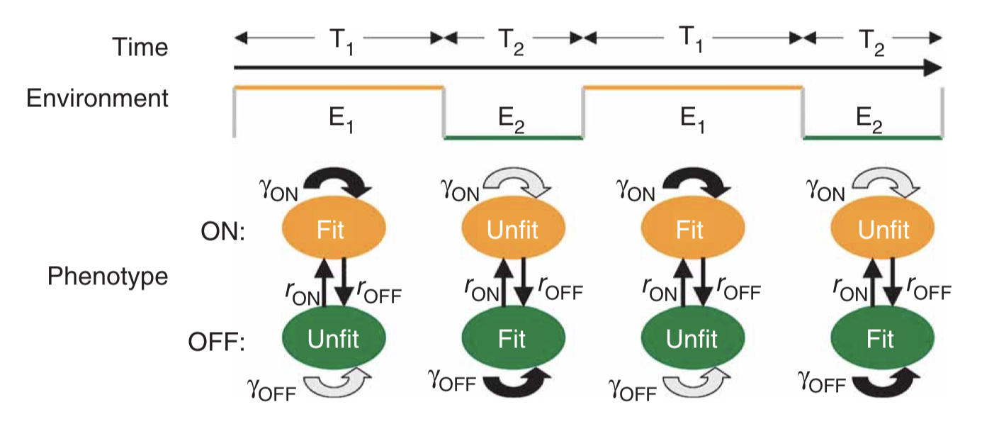
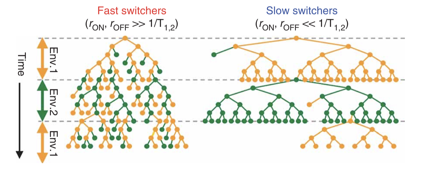
If the cells simply switch randomly between states, then the key physiological parameters are the switching rates, i.e. the probability per unit time that an individual cell switches from one state to the other. If the switching rate of the cell is much faster than the switching rate of the environment, then one would tend to have a mixed population of cells, as shown in the next figure on the left. On the other hand, if the cells switch infrequently compared to the rate of environmental change then one would have the situation on the right:
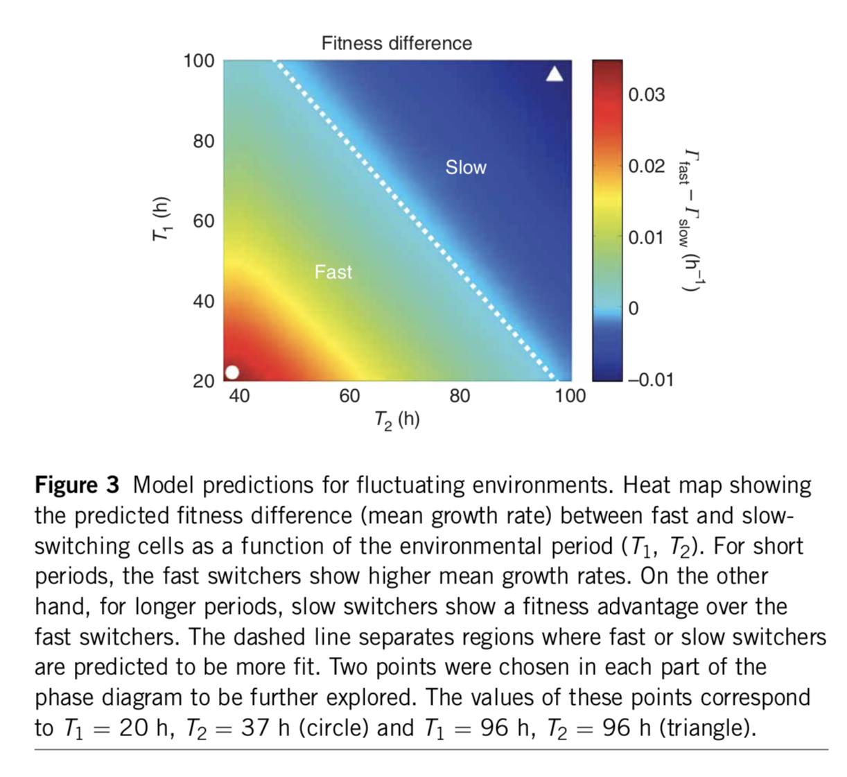
The most basic question one can ask about such a system is: Given the environmental switching rate, and the growth rate (fitness) of each state in each environment, what are the optimal cellular switching rates? To address this question, one can construct a population dynamic model, in which we write down differential equations for the number of cells, or the number of cells in each state, rather than the number of proteins in the cell. Just as proteins can be synthesized and diluted/degraded, so too cells can proliferate and dilute/die. However, note that the rate of proliferation (at least in the exponential growth regime, far below the 'carrying capacity' of the environment), is proportional to the amount of cells one already has, rather than a constant production term as we have for protein expression. We write down a minimal model for two cellular states. For simplicity, we assume a symmetry: state 0 is equally as fit in environment 0 as state 1 is in environment 1. There are then only two (rather than four) growth rates we have to think about: the growth rate of either type of cell in its more ($\gamma_1$) or less ($\gamma_0$) fit environment. The other cellular parameters are the rates of switching from the more fit to the less fit state ($k_0$), or vice versa ($k_1$). \begin{align} \frac{dn_0}{dt} &= \gamma_0(E) n_0 -k_1 n_0 + k_0 n_1 \\[1em] \frac{dn_1}{dt} &= \gamma_1(E) n_1 +k_1 n_0 - k_0 n_1 \end{align} The overall growth rate, which we take to be the fitness, is calculated as the growth rate of the total population size, $n=n_0+n_1$: \begin{align} \gamma &= \frac{1}{n} \frac{dn}{dt} \\[1em] &=\frac {\frac{dn_0}{dt}+\frac{dn_1}{dt}}{n_0+n_1} \end{align} Analyzing this model shows that the optimal switching rate depends, as you might expect, on the switching rates of the environment, as shown here:
An analytical approach enables comparison of responsive and stochastic switching strategies
Kussell and Leibler approached this problem in a general, elegant paper (Science, 2005).
The authors compare responsive and stochastic switching strategies.
Environment dynamics. They imagine a set of different environments, each of which lasts for a random, exponentially distributed, time, followed by a transition to another environmental state. The $i^{th}$ environment has a mean lifetime, $\tau_i$. They further allow a probabilistic alternation among environments, characterized by a matrix of environment switching rates, with $b_{ij}$ denoting the probability of switching to environment $i$ from environment $j$.
Cell state dynamics On the cellular side, they similarly allow a set of distinct physiological states or phenotypes, each of which can, in general, have a specific growth rate in each of the environments. A matrix, $H_{ij}^k$ describes the rate at which state $j$ switches to state $i$ in environment $k$.
For stochastic switching, the $H_{ij}$ values are independent of the environment because, by definition, the cell is simply ignoring the environment.
For responsive switching, the cell can "deliberately" switch to the optimal state in each environment. Without loss of generality, one can choose the fastest growing state in environment $k$ to be the $k^{th}$ state. One can then write that $H_{kj}^{(k)} = H_m$, where $H_m$ is a single switching rate, when $j\ne k$, with all the other $H_{ij}^{k}$ values set to 0. In other words, everyone tries to switch to the best ($k^{th}$) state in each environment.
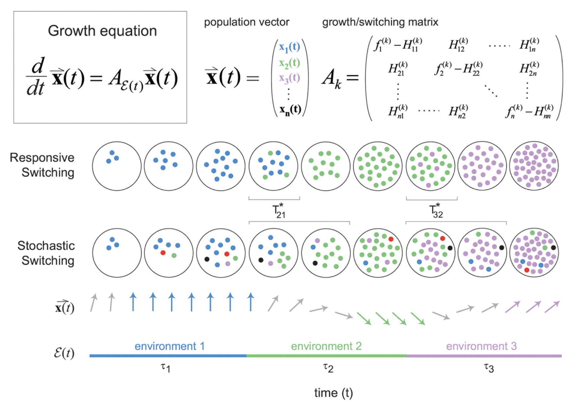
The dynamics are then described by a set of equations for the size of each cell state population, collected together in a cellular state vector, $\vec{x}$. The dynamics of $\vec{x}$ depend in turn on the environments, the switching rates, and the growth rates of each cell state in each environment, all collected together into the matrix $\mathbf{A_k}$ as shown in the diagram above.
\begin{align} \frac{\mathrm{d}\vec{x}}{\mathrm{d}t} = \mathbf{A_k} \vec{x} \end{align}Each strategy incurs a different type of cost:
- Sensing requires a constant cost in the production of the sensing machinery, which is not "paid" by the stochastic switchers.
- The stochastic switching strategy incurs a "diversity cost", due to populating sub-optimal states in each environment.
They derive expressions for the growth rates in the two strategies:
Responsive switching: Long-term growth = Fastest growth - sensing cost - delay time cost
Stochastic switching: Long-term growth = Fastest growth - diversity cost - delay time cost
Note the different costs that are incurred in the two strategies. Generally speaking, sensing is favored when the diversity costs would be high, sensing costs are low, and the environment is highly variable. By contrast, stochastic switching can be favored in regimes in which sensing costs are higher, and environments are stable over longer times. (These statements are made mathematically precise in the paper).
Antibiotic persistence: a stochastic switching strategy
When one adds antibiotics to a bacterial culture, one often finds that they can kill almost, but not quite, all of the cells. A small fraction of cells can survive the antibiotic. Furthermore, these cells turn out to not be resistant mutants. When one grows them up into a new population in the absence of the antibiotic, and then again exposes them to antibiotic, only the same tiny fraction of cells again survive.
Here is a definition of persistence from Allison et al. (Current Opinion in Microbiology, 2011):
Bacterial persistence is a phenomenon in which a sub-population of cells survives antibiotic treatment.... In contrast to resistant bacteria, persisters do not grow in the presence of antibiotics and their tolerance arises from physiological processes rather than genetic mutations... Persistence was first described by Joseph Bigger in 1944 while attempting to sterilize cultures of pathogenic Staphylococcus aureus with penicillin. He found that a small number of cells "persisted" and could later form colonies even after treatment with high antibiotic concentrations.
Persistence is a major problem in many infectious diseases:
- Persistence leads to recurrent infections
- It extends duration of treatments
- It plays an important role in the therapy choice for immunocompromised patients.
- It is important for understanding infections poorly controlled by the immune system, such as tuburculosis.
Persistence is not specific to bacteria. A similar phenomenon allows cancer cells to survive chemotherapeutics. For a recent review, see: Maisonneuve and Gerdes (Cell, 2014).
The general phenomenon is diagrammed here:
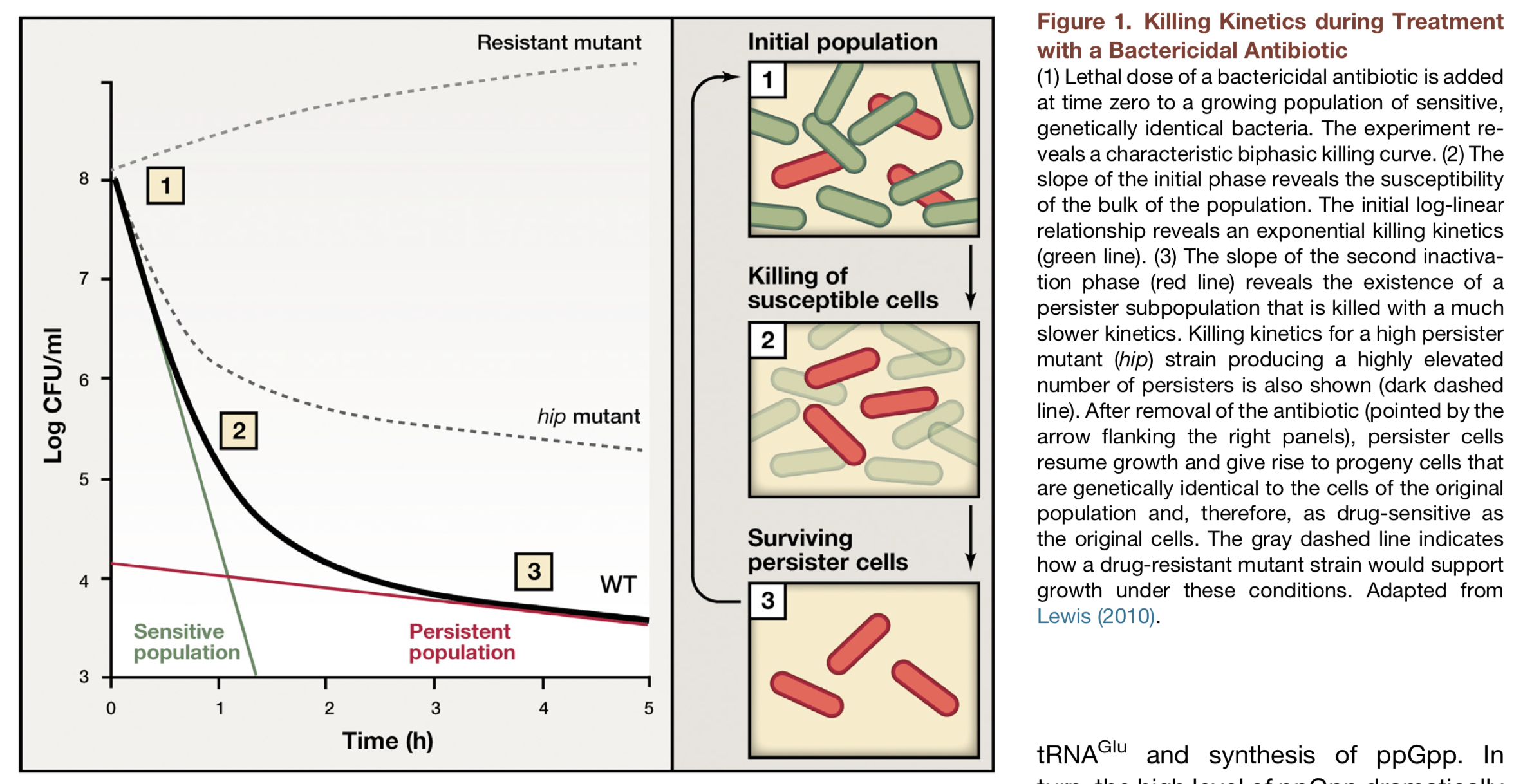
There are different potential explanations for persistence:
- Spatial heterogeneity: aggregates, etc.
- Temporal heterogeneity: adaptive response to the antibiotic
- Pre-existing heterogeneity?
Persistence in movies
The most direct way to visualize persistence is to look at it directly using time-lapse movies. Notice here the large variation in the time at which different cells start growing, even though they are all in essentially the same environment.
Balaban and Leibler (Science, 2004) used a microfluidic approach to film cells before, during, and after antibiotic treatment. The idea was to see whether the persistent state was already present prior to the antibiotic, or whether it was a response, in some cells, to antibiotic addition.
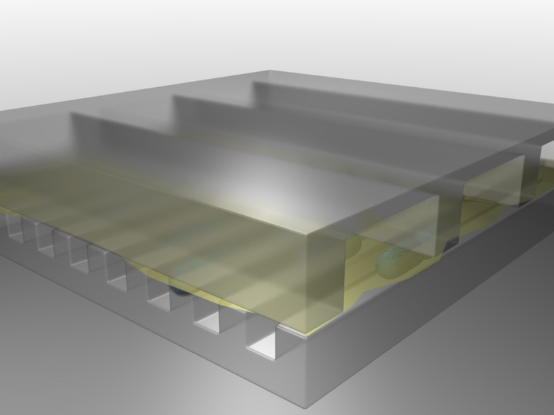
In this device, a predecessor to the mother machine we saw in a previous lesson, bacteria can grow in long channels embedded in PDMS, while media conditions can be rapidly changed. Using this device, one can then watch cells grow before, during, and after addition of an antibiotic, in this case ampicillin:
Here is their diagram of what they saw in the movie:
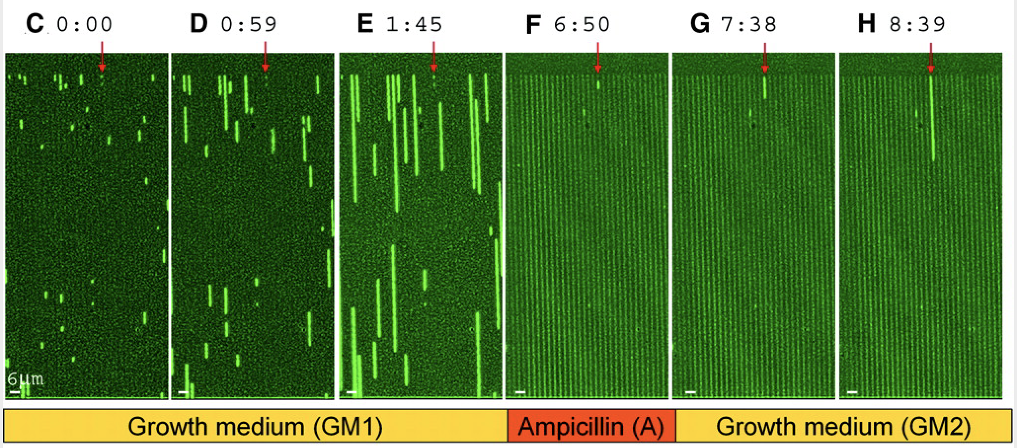
From these experiments, we can see directly that cells spontaneously switch to persistent states characterized by slow growth. These states are far less vulnerable to attack by ampicillin, which affects cell wall synthesis. After removal antibiotics, these cells can resume growth.
Persistence comes in multiple flavors
Through the movies and many other experiments, the authors realized that there are at least two "types" of persisters: Those that are formed in response to a triggering event, termed type I persisters, and those that are formed spontaneously, type II persisters. The difference between the two is whether the transition to the persistent state is spontaneous (type II) or triggered by an environmental condition (type I), summarized in the following reaction scheme:
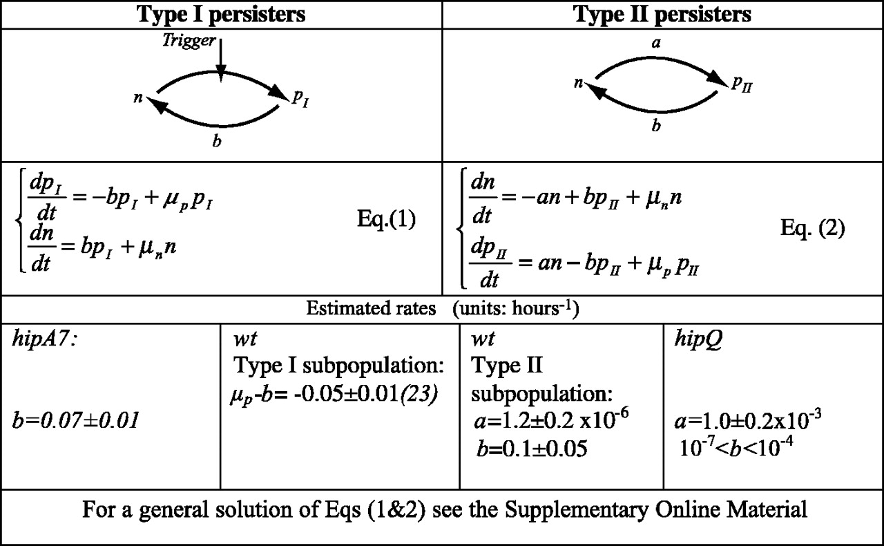
Type I persisters are formed at stationary phase, but not during exponential growth, unlike type II persisters, which form spontaneously even in exponentially growing cultures. From the experiments, they were also able to measure the effective transition rates, as shown above, both for wild-type cells and for so-called "hip" (high incidence of persisters) mutants that generate persisters at elevated frequencies. Interestingly, the two types of persisters do not differ only in the way in which they are generated. It also appeared that type II persisters are not fully growth arrested but rather still grow, albeit an order of magnitude more slowly than normal cells.
Note that subsequent work went on to figure out the mechanism of persister formation and its connection to "toxin-antitoxin" modules that function as ultrasensitive switches through stoichiometric protein-protein interactions!
Summary
- General strategy: given unpredictability in the future environment, “bet” (differentiate) fractions of the population to different states (Kelly betting).
- Stochastic switching can outperform a sense and respond system in some cases (e.g. high sensing costs, low diversity costs).
- Bacterial persistence is an example of a bet-hedging system. In some cases, persisters form prior to antibiotic exposure, but enable survival of antibiotic treatments.
- Toxin-antitoxin cassettes provide a mechanism for ultra sensitive noise-driven switching between persistent and sensitive states.
- In the toxin-antitoxin system, stoichiometric mutual inhibition allows ultrasensitive switching between discrete states.