17. Paradoxical regulation enables bistable homeostatic states (and a review of techniques for dynamical systems)
(c) 2019 Justin Bois and Michael Elowitz. With the exception of pasted graphics, where the source is noted, this work is licensed under a Creative Commons Attribution License CC-BY 4.0. All code contained herein is licensed under an MIT license.
This document was prepared at Caltech with financial support from the Donna and Benjamin M. Rosen Bioengineering Center.

This lesson was generated from a Jupyter notebook. Click the links below for other versions of this lesson.
import numpy as np
import scipy.optimize
import scipy.integrate

import biocircuits

# Plotting modules
import bokeh.io
import bokeh.plotting

notebook_url = 'localhost:8888'
bokeh.io.output_notebook()
In this lesson, we will explore biphasic control of cell populations, in which a molecule is favorable for cell growth at moderate concentrations, but detrimental if in very small or very large concentrations. In doing so, we will review the techniques we have learned for analysis of dynamical systems. We also introduce two new techniques for analysis of dynamical systems: a separatrix and Bendixon's criterion and the Poicaré-Bendixon theorem for analyzing oscillatory circuits.
Biphasic control is a type of paradoxical circuit
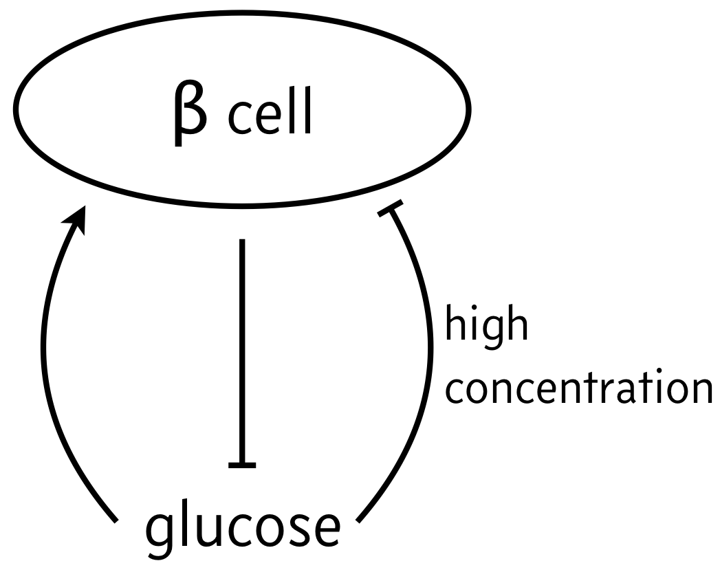
As a classic example of biphasic control, we can think of the relationship between β cells and glucose. In response to elevated glucose levels, β cells secrete insulin, which serves to reduce glucose levels. But if glucose levels get too high, they are toxic to the β cells, which can undergo die off. So, the propensity for β cells to produce insulin (simple noted "β cells" in the schematic below) has is low for both high and low levels of glucose, but high for moderate levels of glucose.
We will investigate the consequences of this circuit architecture in this lesson. In doing so, we will review many of the important techniques from dynamical systems in analyzing biological circuits. This analysis follows closely the results of Karin and Alon, Molec. Sys. Biol., 2017.
Dynamical equations
We model the cellular circuit with a system of ODEs as follows.
\begin{align} \frac{\mathrm{d}c}{\mathrm{d}t} &= (\beta_c(m) - \gamma_c(m))\,c \\[1em] \frac{\mathrm{d}m}{\mathrm{d}t} &= \beta_m - \gamma_m(c)\,m. \end{align}The production and degradation rate of insulin producing β cells are both dependent on the insulin concentration $m$ and are proportional to the cell concentration $c$. This is typically of cellular circuits; the more cells, the greater the proliferation rate. The parameter $\beta_m$ is the feed rate of glucose, which is accomplished in an organism by eating and drinking, or in a cell culture by injection of glucose.
We choose the following forms for the functions above.
\begin{align} \beta_c(m) &= \beta_{c,1}\,\frac{(m/k_\beta)^{n_\beta}}{1 + (m/k_\beta)^{n_\beta}},\\[1em] \gamma_c(m) &= \gamma_{c,0} + \gamma_{c,1}\,\frac{(m/k_\gamma)^{n_\gamma}}{1 + (m/k_\gamma)^{n_\gamma}}, \\[1em] \gamma_m(c) &= \gamma_{m,1}\,c. \end{align}Importantly, in looking at the forms of $\beta_c(m)$ and $\gamma_c(m)$, we see that for small and large $m$, the growth rate $\beta_c(m) - \gamma_c(m)$ is negative, leading to decrease in insulin producing β cells. But for intermediate $m$, we have have positive $\beta_c(m) - \gamma_c(m)$.
We can nondimensionalize defining
\begin{align} &\beta_c = \frac{\beta_{c,1}}{\gamma_{c,0}},\\[1em] &\gamma = \frac{\gamma_{c,1}}{\gamma_{c,0}},\\[1em] &\kappa = \frac{k_\beta}{k_\gamma},\\[1em] &\beta_m \leftarrow \frac{\beta_m}{k_\beta \gamma_{c,0}},\\[1em] &t \leftarrow \gamma_{c,0}t,\\[1em] &m \leftarrow k_\beta m, \\[1em] &c \leftarrow \frac{\gamma_{c,0}}{\gamma_{m,1}}\,c. \end{align}The result is
\begin{align} \frac{\mathrm{d}c}{\mathrm{d}t} & = \left(\beta_c\,\frac{m^{n_\beta}}{1 + m^{n_\beta}} - 1 - \gamma\,\frac{(\kappa m)^{n_\gamma}}{1 + (\kappa m)^{n_\gamma}}\right)c, \\[1em] \frac{\mathrm{d}m}{\mathrm{d}t} &= \beta_m - cm. \end{align}These are the dynamical equations we will study.
Solving numerically
The first technique we learned for the analysis of dynamical system was numerical integration. First, we'll write functions necessary to perform the numerical integration. Note that we are using techniques of modular programming here; we write functions that do single simple tasks.
def acthill(x, kappa, n):
    """Activating Hill function."""
    xkn = (kappa * x)**n
    return xkn / (1 + xkn)


def dc_dt(c, m, beta_c, gamma, kappa, n_beta, n_gamma):
    return (beta_c * acthill(m, 1, n_beta)
            - 1 - gamma * acthill(m, kappa, n_gamma)) * c


def dm_dt(c, m, beta_m):
    return beta_m - c * m


def ode_rhs(x, t, beta_m, beta_c, gamma, kappa, n_beta, n_gamma):
    """Compute right-hand-side of pair of ODEs."""
    c, m = x
    return np.array([dc_dt(c, m, beta_c, gamma, kappa, n_beta, n_gamma),
                     dm_dt(c, m, beta_m)])
Let's integrate, and see what happens, starting at two different initial concentrations of cells , both with a dimensionless glucose level of 1/2. We take the parameter values from the Karin and Alon paper.
# Specify parameters
beta_m = 3.79
beta_c = 16.0
gamma = 20.0
kappa = 0.875
n_beta = 6
n_gamma = 6

# Package for the integrating function
params_c = (beta_c, gamma, kappa, n_beta, n_gamma)
params_m = (beta_m,)
params = params_m + params_c

# Set up initial condition and solve
x0 = np.array([2, 0.5])
t = np.linspace(0, 3, 400)
x_low = scipy.integrate.odeint(ode_rhs, x0, t, args=params)

# And again with higher initial condition
x0 = np.array([5, 0.5])
x_high = scipy.integrate.odeint(ode_rhs, x0, t, args=params)

# Plot the result
p = bokeh.plotting.figure(width=450, height=300, x_axis_label='time')
p.line(t, x_low[:,0], line_width=2, legend='cells')
p.line(t, x_low[:,1], line_width=2, color='orange', legend='glucose')
p.line(t, x_high[:,0], line_width=2, line_dash='dashed')
p.line(t, x_high[:,1], line_width=2, color='orange', line_dash='dashed')
p.legend.location = 'top_left'

bokeh.io.show(p)
When the number of β cells producing insulin is initiall low, the cells stop producing insulin and the glucose concentration grows to high levels, a "diabetes condition." Conversely, when the numebr of β cells producing insulin is higher, they stablize and maintain a consistent insulin level.
Plotting the phase portrait
We can solve for various parameter values,and can even make interactive plots where we vary initial conditions, but a phase portrait provides a concise view into the system dynamics from various starting points.
First, we will plot the flow of the dynamical system.
c_range = [1, 7]
m_range = [0, 2]

p = biocircuits.phase_portrait(dc_dt,
                               dm_dt,
                               c_range,
                               m_range,
                               params_c,
                               params_m,
                               x_axis_label='c',
                               y_axis_label='m',
                               color='#e6ab02',
                               plot_width=350)

bokeh.io.show(p)
Next, we add the nullclines. The $m$-nullcline is easy to compute. We solve
\begin{align} \frac{\mathrm{d}m}{\mathrm{d}t} = \beta_m - c m = 0, \end{align}which gives
\begin{align} m = \frac{\beta_m}{c}. \end{align}The $c$-nullcline is more challenging. We need to solve
\begin{align} \frac{\mathrm{d}c}{\mathrm{d}t} & = \left(\beta_c\,\frac{m^{n_\beta}}{1 + m^{n_\beta}} - 1 - \gamma\,\frac{(\kappa m)^{n_\gamma}}{1 + (\kappa m)^{n_\gamma}}\right)c = 0. \end{align}An obvious solution is $c = 0$. The means there is a vertical nullcline along the $m$-axis in the $x$-$m$ plane. There may be horizontal lines (fixed $m$, nonzero $c$) where
\begin{align} f(m) \equiv \beta_c\,\frac{m^{n_\beta}}{1 + m^{n_\beta}} - 1 - \gamma\,\frac{(\kappa m)^{n_\gamma}}{1 + (\kappa m)^{n_\gamma}} = 0. \end{align}This can be rewritten as
\begin{align} \beta_c\,\frac{m^{n_\beta}}{1 + m^{n_\beta}} = 1 + \gamma\,\frac{(\kappa m)^{n_\gamma}}{1 + (\kappa m)^{n_\gamma}}. \end{align}Both the right-hand-side and left-hand-side are monotonically increasing functions of $m$. Each side also has a single inflection point and asymptotes to a finite value. The right-hand-side starts above the left-hand-side at $m=0$. Therefore the lines represented by either side of this equation may cross zero, one, or two times, depending on the parameters. Therefore, there are either zero, one, or two horizontal lines in the $c$-nullcline.
To find the values of $m$ for which we have a horizontal line for the $c$-nullcline, we need to find the roots of $f(m)$. As is often the case with root finding, there are many ways to do it, and some work better than others. Our strategy here is to brute-force find the places where the $f(m)$ curve crosses the $m$-axis by gridding up the axis and evaluating the sign of $f(m)$ at each point. Wherever the sign changes, we know the function crossed the $m$-axis. We then hone in on the root near a crossing point using Brent's method. We code this up below.
def growth_rate(m, beta_c, gamma, kappa, n_beta, n_gamma):
    """Growth rate, f(m), of β cells"""
    return dc_dt(1, m, beta_c, gamma, kappa, n_beta, n_gamma)


def dc_dt_nullclines(m_range, beta_c, gamma, kappa, n_beta, n_gamma):
    """Determine values for horizontal nullclines."""
    # Brute force to guess how many roots
    m = np.linspace(m_range[0], m_range[1], 1000)
    sgn = growth_rate(m, beta_c, gamma, kappa, n_beta, n_gamma) > 0
    switches = np.where(np.diff(sgn))
    args = (beta_c, gamma, kappa, n_beta, n_gamma)

    # Hone in on each root
    return np.array([scipy.optimize.brentq(growth_rate, m[i-1], m[i+1], args=args)
                for i in switches[0]])


def plot_nullclines(c_range, m_range, beta_m, beta_c, gamma, kappa, n_beta, n_gamma, p):
    # dm/dt = 0 nullcline
    c = np.linspace(*c_range, 200)
    p.line(c, beta_m/c, line_width=2, color='#7570b3')

    # dc/dt = 0 nullcline
    m_vals = dc_dt_nullclines(m_range, beta_c, gamma, kappa, n_beta, n_gamma)
    for m in m_vals:
        p.ray(0, m, length=0, angle=0, line_width=2, color='#1b9e77')
    p.ray(0, 0, length=0, angle=np.pi/2, line_width=2, color='#1b9e77')

    return p


# Add nullclines to the phase portrait
p = plot_nullclines(c_range, m_range, beta_m, beta_c, gamma, kappa, n_beta, n_gamma, p)

bokeh.io.show(p)
Finding and characterizing fixed points
The fixed points are where the nullclines cross. Since we know the values of $m$ for which the $c$-nullcline is horizontal (we found them numerically), we can use them to get the value of $c$ for a fixed point via $c = \beta_m/m$.
def fixed_points(c_range, m_range, beta_m, beta_c, gamma, kappa, n_beta, n_gamma):
    """Give all fixed points with a given range"""
    m = dc_dt_nullclines(m_range, beta_c, gamma, kappa, n_beta, n_gamma)
    c = beta_m / m

    return np.array([[c_val, m_val] for c_val, m_val in zip(c, m)])
In addition to finding the fixed points, we need to characterize them as being stable or unstable. To that end, we can perform a linear stability analysis. We expand the system of ODEs in a Taylor series about a fixed point $(c_0, m_0)$, keeping only terms to first order in the perturbations $\delta m$ and $\delta c$. Note that this means we do not keep terms of oder $\delta m \delta c$.
\begin{align} &\frac{\mathrm{d}\delta c}{\mathrm{d} t} = \left(\beta_c\,\frac{m_0^{n_\beta}}{1 + m_0^{n_\beta}} - 1 - \gamma\,\frac{(\kappa m_0)^{n_\gamma}}{1 + (\kappa m_0)^{n_\gamma}}\right)\delta c + c_0\left(\beta_c\,\frac{n_\beta m_0^{n_\beta-1}}{(1+m_0^{n_\beta})^2} - \gamma\,\frac{n_\gamma (\kappa m_0)^{n_\gamma}}{m_0(1+(\kappa m_0)^{n_\gamma})^2}\right)\delta m ,\\[1em] &\frac{\mathrm{d}\delta m}{\mathrm{d} t} = -m_0\, \delta c - c_0\,\delta m. \end{align}This gives a linear stability matrix of
\begin{align} \mathsf{A} = \begin{pmatrix} \beta_c\,\frac{m_0^{n_\beta}}{1 + m_0^{n_\beta}} - 1 - \gamma\,\frac{(\kappa m_0)^{n_\gamma}}{1 + (\kappa m_0)^{n_\gamma}} & c_0\left(\beta_c\,\frac{n_\beta m_0^{n_\beta-1}}{(1+m_0^{n_\beta})^2} - \gamma\,\frac{n_\gamma (\kappa m_0)^{n_\gamma}}{m_0(1+(\kappa m_0)^{n_\gamma})^2}\right) \\[1em] -m_0 & -c_0 \end{pmatrix}. \end{align}While we could analytically compute the eigenvalues for this matrix, it would not do us much good, as the expression is very messy. Rather, we will compute the eigenvalues and eigenvectors numerically for the fixed points, which we found numerically anyway.
def acthill_deriv(x, kappa, n):
    xkn = (kappa * x)**n
    return n * xkn / x / (1 + xkn)**2


def lin_stab_matrix(c0, m0, beta_m, beta_c, gamma, kappa, n_beta, n_gamma):
    """Compute linear stability matrix for a fixed point."""
    A = np.empty((2, 2))
    A[0,0] = beta_c * acthill(m0, 1, n_beta) - 1 - gamma * acthill(m0, kappa, n_gamma)
    A[0,1] = c0*(beta_c * acthill_deriv(m0, 1, n_beta)
                 - gamma * acthill_deriv(m0, kappa, n_gamma))
    A[1,0] = -m0
    A[1,1] = -c0

    return A


def lin_stab(c0, m0, beta_m, beta_c, gamma, kappa, n_beta, n_gamma):
    """Perform linear stability analysis for a given fixed point.
    Returns eigenvalues and eigenvectors of fixed point.
    """
    A = lin_stab_matrix(c0, m0, beta_m, beta_c, gamma, kappa, n_beta, n_gamma)

    return np.linalg.eig(A)
We can use the eigenvalues to determine the stability of a fixed point. We plot unstable fixed points with open circles and stable ones with closed circles.
def plot_fixed_points(c_range, m_range, beta_m, beta_c, gamma, kappa, n_beta, n_gamma, p):
    """Plot fixed points, closed = stable, open = unstable"""
    fps = fixed_points(c_range, m_range, beta_m, beta_c, gamma, kappa, n_beta, n_gamma)
    for fp in fps:
        evals, evecs = lin_stab(*fp, beta_m, beta_c, gamma, kappa, n_beta, n_gamma)
        if (evals.real < 0).all():
            fill_color = 'black'
        else:
            fill_color='white'

        p.circle(*fp, size=7, line_width=2,
                 fill_color=fill_color, line_color='black')

    return p


# Add fixed points to the phase portrait
p = plot_fixed_points(c_range, m_range, beta_m, beta_c, gamma, kappa, n_beta, n_gamma, p)

bokeh.io.show(p)
Plotting the separatrix
In looking at the phase portrait, if we start with $c = 2$ and $m = 1/2$, the system carries us away toward the diabetic state with runaway glucose and no β cells producing insulin. Conversely, if we start with $c=5$ and $m=1/2$, the system progresses toward the stable fixed point. In moving from $c = 2$ to $c = 5$, we have crossed a separatrix. The qualitative behavior of the system changes by crossing that line.
The separatrix goes through the unstable fixed point, which is a saddle. A saddle has one positive eigenvalue, but the other eigenvalues are negative. The system is thus attracted to the saddle fixed point along the eigenvector corresponding to the negative eigenvalue, before pushing away from the fixed point along the eigenvector corresponding to the positive eigenvalue.
To plot the separatrix, we can start at the unstable fixed point, and then take a tiny step along the eigenvector corresponding to the negative eigenvalue. We will call this eigenvector $\mathbf{v}$. We then integrate the dynamical system backwards in time to generate the separatrix. This enables us to trace out the path that attracts the system toward the saddle. We can do the same thing stepping just off of the saddle fixed point in the $-\mathbf{v}$ direction. This enables use to plot a separatrix separating dynamics that go right toward the stable fixed point or left toward runaway glucose.
def plot_separatrix(c0, m0, c_range, m_range, beta_m, beta_c, gamma, kappa, n_beta, n_gamma,
                    p, t_max=3, eps=1e-6, color='#d95f02', line_width=2):
    """
    Plot separatrix on phase portrait.
    """
    # Negative time function to integrate to compute separatrix
    def rhs(x, t):
        # Unpack variables
        c, m = x

        # Stop integrating if we get the edge of where we want to integrate
        if c_range[0] < c < c_range[1] and m_range[0] < m < m_range[1]:
            return -ode_rhs(x, t, beta_m, beta_c, gamma, kappa, n_beta, n_gamma)
        else:
            return np.array([0, 0])

    # Compute eigenvalues and eigenvectors
    evals, evecs = lin_stab(c0, m0, beta_m, beta_c, gamma, kappa, n_beta, n_gamma)

    # Get eigenvector corresponding to attraction
    evec = evecs[:, evals<0].flatten()

    # Parameters for building separatrix
    t = np.linspace(0, t_max, 400)

    # Build upper right branch of separatrix
    x0 = np.array([c0, m0]) + eps * evec
    x_upper = scipy.integrate.odeint(rhs, x0, t)

    # Build lower left branch of separatrix
    x0 = np.array([c0, m0]) - eps * evec
    x_lower = scipy.integrate.odeint(rhs, x0, t)

    # Concatenate, reversing lower so points are sequential
    sep_c = np.concatenate((x_lower[::-1,0], x_upper[:,0]))
    sep_m = np.concatenate((x_lower[::-1,1], x_upper[:,1]))

    # Plot
    p.line(sep_c, sep_m, color=color, line_width=line_width)

    return p
Now that we have the code, we start at the unstable fixed point.
fp = fixed_points(c_range, m_range, beta_m, beta_c, gamma, kappa, n_beta, n_gamma)
fp = fp[1]

p = plot_separatrix(*fp, c_range, m_range, beta_m, beta_c,
                    gamma, kappa, n_beta, n_gamma, p)

bokeh.io.show(p)
To recap (and to make a prettier plot with appropriate layering), we can build this annotated phase portrait in stages.
p = biocircuits.phase_portrait(dc_dt,
                               dm_dt,
                               c_range,
                               m_range,
                               params_c,
                               params_m,
                               x_axis_label='c',
                               y_axis_label='m',
                               color='#e6ab02',
                               plot_width=350)

p = plot_nullclines(c_range, m_range, beta_m, beta_c, gamma, kappa, n_beta, n_gamma, p)

p = plot_separatrix(*fp, c_range, m_range, beta_m, beta_c,
                    gamma, kappa, n_beta, n_gamma, p)

p = plot_fixed_points(c_range, m_range, beta_m, beta_c, gamma, kappa, n_beta, n_gamma, p)

bokeh.io.show(p)
The system is more robust to fluctuations in glucose levels if the fixed points are farther apart
The more you can spread apart the fixed points, the more robust to fluctuations in glucose levels the system is. That is, it will avoid jumping off toward the runaway glucose state the farther apart the fixed points are. We can see how the system parameters affect the spread of fixed points be plotting the growth rate,
\begin{align} \beta_c\,\frac{m^{n_\beta}}{1 + m^{n_\beta}} - 1 - \gamma\,\frac{(\kappa m)^{n_\gamma}}{1 + (\kappa m)^{n_\gamma}}, \end{align}for various parameter values.
The plot below will not appear in the HTML version of this notebook.
slider_params = (biocircuits.AttributeContainer(title='βc', start=1,
                                                end=50, value=16, step=0.05),
                 biocircuits.AttributeContainer(title='γ', start=1,
                                                end=50, value=20, step=0.05),
                 biocircuits.AttributeContainer(title='κ', start=0.05,
                                                end=1, value=0.85, step=0.05),
                 biocircuits.AttributeContainer(title='nβ', start=1,
                                                end=10, value=6, step=0.05),
                 biocircuits.AttributeContainer(title='nγ', start=1,
                                                end=10, value=6, step=0.05),)


def callback(source, x_range, y_range, sliders, toggles):
    beta_c, gamma, kappa, n_beta, n_gamma = tuple(slider.value for slider in sliders)

    # Compute net production
    m = np.linspace(0, x_range.end, 400)
    source.data['m'] = m
    source.data['net_prod'] = growth_rate(m, beta_c, gamma, kappa, n_beta, n_gamma)
    source.data['zero_line'] = np.zeros_like(m)


def net_prod_plot(callback, sliders, toggles, extra_args):
    # Set up plot
    p = bokeh.plotting.figure(plot_width=500,
                              plot_height=300,
                              x_axis_label='m',
                              y_axis_label='fractional net production')

    # Set up empty data source
    source = bokeh.models.ColumnDataSource()

    # Populate glyphs
    p.line('m', 'net_prod', source=source, line_width=2)
    p.line('m', 'zero_line', source=source, color='black')

    # Update data according to callback
    callback(source, bokeh.models.Range1d(0, 10), None,
             sliders, toggles, *extra_args)

    return p, source

# Build the interactive plotting app
app = biocircuits.interactive_xy_plot(net_prod_plot, callback,
                                      slider_params, (), ())

# Show the app
bokeh.io.show(app, notebook_url=notebook_url)
We find the the parameter $\kappa = k_\beta/k_\gamma$ has the largest effect. this matches intuition; a higher threshold for for glucotoxicity results in a the system being more robust to fluctuations in glucose levels.
Identification of oscillations
So far in this lesson, we have seen how tools from dynamical systems allow us to investigate how circuits may respond to perturbation, even in qualitative ways like when we cross a separatrix. We now introduce some more useful notions from dynamical systems.
We briefly mentioned that there are some general ways to identify dynamical systems that can undergo oscillations. We will now discuss a couple of very powerful theorems for two-dimensional systems. We state both without proof.
Bendixson's criterion
This theorem makes it possible to rule out sustained oscillations (defined as orbits, closed curves on which trajectories remain after entering).
Consider a dynamical system
\begin{align} \dot{x} = f(x, y)\\[1em] \dot{y} = g(x,y). \end{align}In a simply connected region $D$ of the $x$-$y$ plane, if the quantity
\begin{align} \frac{\partial f}{\partial x} + \frac{\partial g}{\partial y} \end{align}is nonzero and does not change sign on $D$, then the dynamical system has no orbits entirely in $D$. To illustrate the power of this, I really like the following exercise from Del Vecchio and Murray's book in which they ask you to eliminate circuits below that cannot have sustained oscillations by using Bendixson's criterion. (Image below, (c) Princeton University Press.)
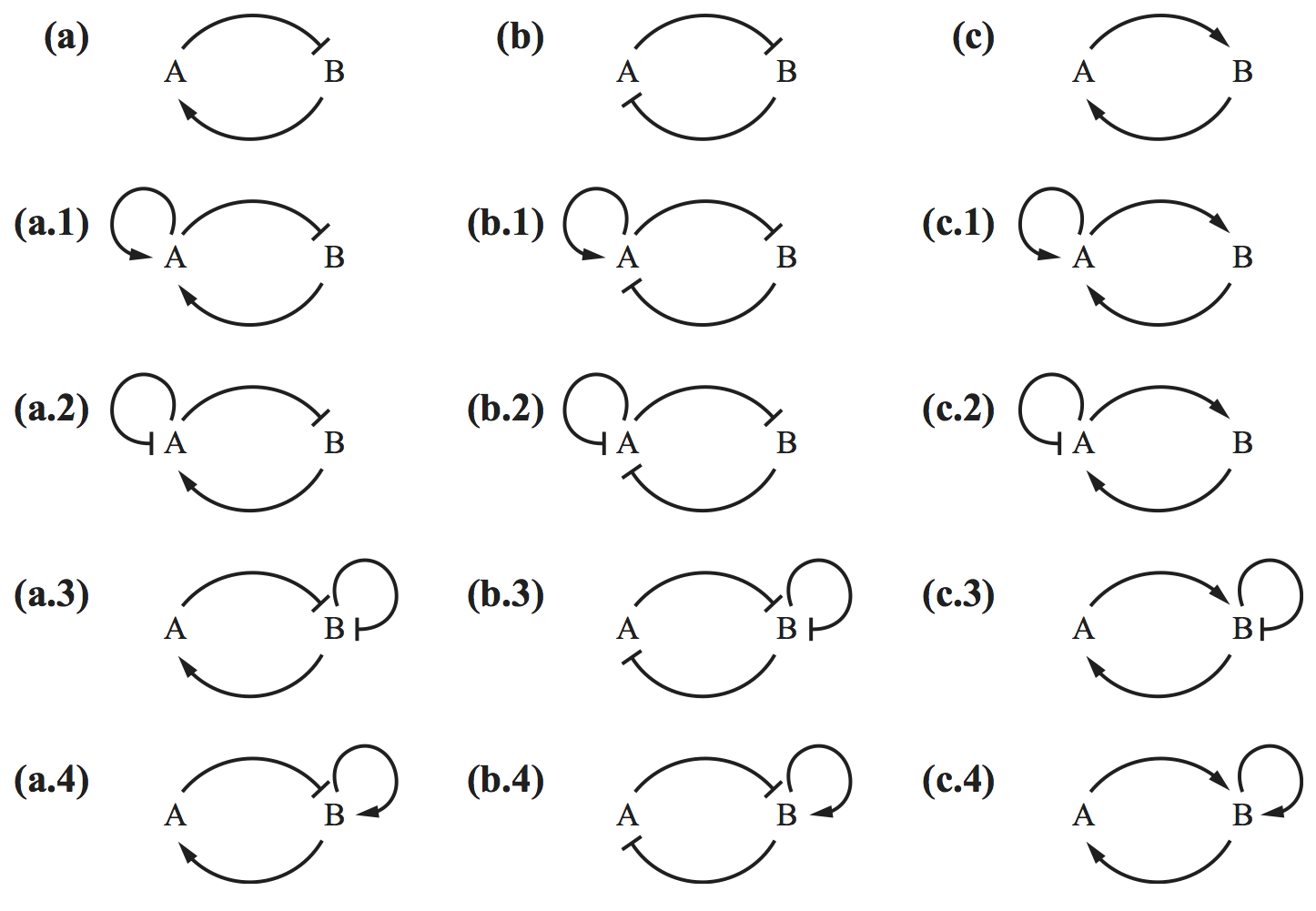
We leave it as an exercise for you think think about which circuits cannot have oscillations.
Poincaré-Bendixson Theorem
We will not state the full theorem here, which involves $\omega$ limit sets, but will instead state important consequences.
- If a two-dimensional dynamical system has no fixed points, it has a periodic solution.
- If a two-dimensional dynamical system has only one unstable fixed point that is not a saddle, it has a periodic solution.
This is useful to decide for what parameter values a system that can potentially oscillate may actually do so.