18. Molecular titration generates ultrasensitive responses in biological circuits
(c) 2019 Justin Bois and Michael Elowitz. With the exception of pasted graphics, where the source is noted, this work is licensed under a Creative Commons Attribution License CC-BY 4.0. All code contained herein is licensed under an MIT license.
This document was prepared at Caltech with financial support from the Donna and Benjamin M. Rosen Bioengineering Center.

This lesson was generated from a Jupyter notebook. Click the links below for other versions of this lesson.
Design principle
- Molecular titration creates ultrasensitive switches and promotes unidirectional communication
Techniques
#### Papers
- N.E. Buchler and M. Louis, Molecular Titration and Ultrasensitivity in Regulatory Networks, J.M.B. (2008).
- N.E. Bucher and F.R. Cross, Protein sequestration generates a flexible ultrasensitive response in a genetic network, Mol. Syst. Biol. (2009).
- S. Mukherji et al, “MicroRNAs can generate thresholds in target gene expression”, Nat. Gen. 2011
- Levine et al, PLoS Biol, 2007; Mukherji et al, 2011: Regulation of mRNA level by small RNAs
- D. Sprinzak et al, Nature 2010; D. Sprinzak et al, PLoS Comput. Biol. 2011
- E. Rotem et al, Regulation of phenotypic variability by a threshold- based mechanism underlies bacterial persistence, PNAS 2010.
- See also: F. Corson et al, “Self-organized Notch dynamics generate stereotyped sensory organ patterns in Drosophila,” Science 2017
import numpy as np
import scipy.stats as st
import numba

import biocircuits

import bokeh.io
import bokeh.plotting

bokeh.io.output_notebook()
Ultrasensitivity is necessary for many circuits - how can one generate it?
Ultrasensitivity plays a key role in many circuits. For example, together with positive feedback, it enables multistability. Together with negative feedback, it enables oscillations.
Ultrasensitive can occur at different levels: for instance, in the transcriptional regulation of a target gene, or in the allosteric regulation of a protein.
Are there simple, generalizable design strategies that could confer ultrasensitivity?
More specifically: If you needed to ensure an ultrasensitive relationship between one species and its target, how would you do it?
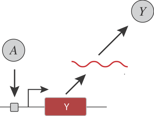
Before we go on, consider a simple gene regulatory system, in which an input activator, $A$, controls the expression of a target protein $Y$:
Let's pause to ask:
- How could you insert ultrasensitivity into the dependence of Y on A?
- How could you make the threshold and sensitivity of the overall input function tunable?
"Subtraction" by titration
Today we will discuss molecular titration, a simple and general mechanism that provides tunable ultrasensitivity across diverse natural systems, and allows engineering of ultrasensitive responses in synthetic circuits.
One of the most striking features of biological molecules is their tendency to form strong and specific complexes with one another. Depending on the system, the complex itself may provide a particular activity, such as gene regulation. Or, alternatively, one of the monomers may provide an activity, with the complex inhibiting it.
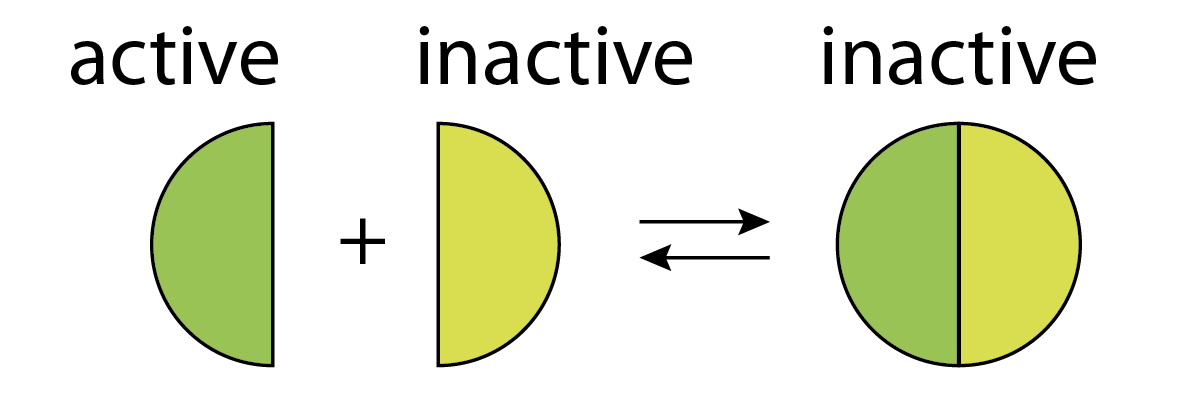
In this example, molecular titration performs a kind of "subtraction" operation, in which an inhibitor (inactive species) "subtracts off" a fraction of otherwise active molecules.
Molecular titration occurs in diverse contexts:
In bacterial gene regulation, specialized transcription factors called sigma factors are stoichiometrically inhibited by cognate anti-sigma factors.
Transcription factors, such as basic helix-loop-helix proteins, form specific homo- and hetero-dimeric complexes with one another, each with a distinct binding specificity or activity.
Small RNA regulators can bind to cognate target mRNAs, inhibiting their translation.
In toxin-antitoxin systems, the "anti-toxin" protein can bind to its cognate toxin, blocking its activity.
Intercellular communication systems often work through direct complexes between ligands and receptors or ligands and inhibitors.
Today we will discuss the way in which these systems use molecular titration, through complex formation, to generate ultrasensitivity.
Molecular titration: a minimal model
To see how molecular titration produces ultrasensitivity we will consider the simplest possible example of two proteins, $A$ and $B$, that can bind to form a complex, $C$, that is inactive for both $A$ and $B$ activities. This system can be described by the following reactions:
$ A + B \underset{k_{\it{off}}}{\stackrel{k_\it{on}}{\rightleftharpoons}} C $
At steady-state we have:
$ k_\it{on} A B = k_\it{off} C $
with
$K_d = k_\it{off}/k_\it{on} = A B / C$
We also will insist on conservation of mass:
\begin{align} A_T = A + C \\ B_T = B + C \end{align}Here, $A_T$ and $B_T$ denote the total amounts of $A$ and $B$, respectively.
From these equations, one can determine an expression for the amount of free $A$ (or $B$) as a function of $A_T$ and $B_T$ for different parameter values:
\begin{align} A = \frac{1}{2} \left( A_T-B_T-K_d+\sqrt{(A_T-B_T-K_d)^2+4A_T K_d} \right) \end{align}What does this relationship look like? More specifically, let's consider a case in which we control the total amount of $A_T$ and see how much free $A$ we get, for different amounts of $B_T$. We will start by assuming the limit of very strong binding (small values of $K_d$):
# array of A_total values
AT = np.logspace(-2, 5, 1001)
Kd = 0.001
BTvals = np.logspace(-1, 3, 5)

# Decide on your color palette
colors = bokeh.palettes.Blues9[3:8][::-1]

p = bokeh.plotting.figure(width=450, height=300,
                         x_axis_label='A_T', y_axis_label='A',
                         x_axis_type="log", y_axis_type="log",
                         title = "A vs. A_T for different values of B_T, in strong binding regime, Kd<<1",
                         x_range=[AT.min(), AT.max()])

# Loop through colors and BT values (nditer not necessary)
A = np.zeros((BTvals.size, AT.size))
p.circle(0, 0, size=0.00000001, color= "#ffffff", legend="B_T")
for i, (color, BT) in enumerate(zip(colors, BTvals)):
   A0 = 0.5 * (AT-BT-Kd+np.sqrt((AT-BT-Kd)**2+4*AT*Kd))
   A[i,:] = A0
   p.line(AT, A0, line_width=2, color=color, legend=str(BT))

p.legend.location = "bottom_right"

bokeh.io.show(p)
The key feature to notice here is that A goes through a very sharp transition from a low to a high value just as $A_T$ reaches $B_T$.
Perhaps it is simpler to view this behavior on a linear axis:
# array of A_total values
AT = np.linspace(0, 200, 1001)
Kd = 0.001
BTvals = 100*np.ones(1)

colors = bokeh.palettes.Blues3[::]

p = bokeh.plotting.figure(width=400, height=300,
                         x_axis_label='A_T', y_axis_label='A',
                         x_axis_type="linear", y_axis_type="linear",
                         title = "A vs. A_T",
                         x_range=[AT.min(), AT.max()])

# Loop through colors and BT values (nditer not necessary)
A = np.zeros((BTvals.size, AT.size))
p.circle(0, 0, size=0.00000001, color= "#ffffff", legend="B_T")
for i, (color, BT) in enumerate(zip(colors, BTvals)):
   A0 = 0.5 * (AT-BT-Kd+np.sqrt((AT-BT-Kd)**2+4*AT*Kd))
   A[i,:] = A0
   p.line(AT, A0, line_width=2, color=color, legend=str(BT))

p.legend.location = "top_left"

bokeh.io.show(p)
Here we see that $A$ is essentially 0 when $A_T < B_T$, and then increases linearly beyond that threshold, becoming approximately proportional to the difference $A_T-B_T$. This is called a threshold-linear relationship.
So far, we have looked in the "strong" binding limit, $K_d<<1$. But any real system will have a finite rate of unbinding. It is therefore important to see how the system behaves across a range of $K_d$ values.
# array of A_total values
AT = np.logspace(-2, 3, 1001)
BT = 1
Kdvals = np.logspace(-3, 1, 5)

# Decide on your color palette
colors = bokeh.palettes.Blues9[3:8][::-1]

p = bokeh.plotting.figure(width=400, height=300,
                         x_axis_label='A_T', y_axis_label='A',
                         x_axis_type="log", y_axis_type="log",
                         title = "A vs. A_T for different values of Kd, B_T=1",
                         x_range=[AT.min(), AT.max()])


# Loop through colors and BT values (nditer not necessary)
A = np.zeros((Kdvals.size, AT.size))
p.circle(0, 0, size=0.00000001, color= "#ffffff", legend="K_d")
for i, (color, Kd) in enumerate(zip(colors, Kdvals)):
   A0 = 0.5 * (AT-BT-Kd+np.sqrt((AT-BT-Kd)**2+4*AT*Kd))
   A[i,:] = A0
   p.line(AT, A0, line_width=2, color=color, legend=str(Kd))

p.legend.location = "bottom_right"
bokeh.io.show(p)
On a linear scale, zooming in around the transition point, we can see that weaker binding "softens" the transition from flat to linear behavior:
# array of A_total values
AT = np.linspace(50, 150, 1001)
Kdvals = np.array([0.01, 0.1,0.5,1])
BT = 100

colors = bokeh.palettes.Blues8[::]

p = bokeh.plotting.figure(width=400, height=300,
                         x_axis_label='A_T', y_axis_label='A',
                         x_axis_type="linear", y_axis_type="linear",
                         title = "A vs. A_T for different K_d values",
                         x_range=[AT.min(), AT.max()])

# Loop through colors and BT values (nditer not necessary)
A = np.zeros((Kdvals.size, AT.size))
p.circle(0, 0, size=0.00000001, color= "#ffffff", legend="Kd")
for i, (color, Kd) in enumerate(zip(colors, Kdvals)):
   A0 = 0.5 * (AT-BT-Kd+np.sqrt((AT-BT-Kd)**2+4*AT*Kd))
   A[i,:] = A0
   p.line(AT, A0, line_width=2, color=color, legend=str(Kd))

p.legend.location = "top_left"

bokeh.io.show(p)
Ultrasensitivity in threshold-linear response functions
Threshold-linear responses differ qualitatively from what we had with a Hill function. Unlike the sigmoidal, or "S-shaped," Hill function, which saturates at a maximum "ceiling," the threshold-linear function increases without bound, maintaining a constant slope as input values increase.
Despite these differences, we can still quantify the sensitivity of this response. A simple way to define sensitivity is the fold change in output for a given fold change in input, evaluated at a particular operating point. The plots below show this sensitivity, $S=\frac{d log A}{d log A_T}$ plotted for varying $A_T$, and for different values of $K_d$. Note the peak in $S$ right around the transition, whose strength grows with tighter binding (lower $K_d$).
# array of A_total values, base 2
AT = np.logspace(-5, 5, 1001 ,base=2)
Kdvals = np.array([0.00001, 0.0001, 0.001,0.01,0.1])
BT = 1

# Color palettes:
colors = bokeh.palettes.Blues9[:][::]
scolors = bokeh.palettes.Oranges9[:][::]

pA = bokeh.plotting.figure(width=400, height=200,
                         x_axis_label='A_T', y_axis_label='A',
                         x_axis_type="log", y_axis_type="log",
                         title = "A vs A_T for several K_d",
                         x_range=[AT.min(), AT.max()])

pS = bokeh.plotting.figure(width=400, height=200,
                         x_axis_label='A_T', y_axis_label='S',
                         x_axis_type="log", y_axis_type="log",
                         title = "Sensitivity vs. A_T for several K_d",
                         x_range=[AT.min(), AT.max()])

# Loop through colors and BT values (nditer not necessary)
A = np.zeros((Kdvals.size, AT.size)) # store A values
S = np.zeros((Kdvals.size, AT.size-1)) #sensitivities are derivatives, so there is one fewer of them
foldstep = AT[1]/AT[0]
pA.circle(0, 0, size=0.00000001, color= "#ffffff", legend="Kd")
pS.circle(0, 0, size=0.00000001, color= "#ffffff", legend="Kd")
for i, (color, scolor, Kd) in enumerate(zip(colors, scolors, Kdvals)):
    A0 = 0.5 * (AT-BT-Kd+np.sqrt((AT-BT-Kd)**2+4*AT*Kd))
    A[i,:] = A0
    pA.line(AT, A0, line_width=2, color=color,legend=str(Kd))

    # define Sensitivity, S, as dlog(A)/dlog(AT)=AT/A*dA/d(AT)
    S0 = AT[0:-2]/A[i,0:-2]*(A[i,1:-1]-A[i,0:-2])/(AT[1:-1]-AT[0:-2])
    pS.line(AT[0:-2],S0,line_width=2,color=scolor,legend=str(Kd))

pA.legend.location = "bottom_right"
pS.legend.location = "bottom_right"

bokeh.io.show(bokeh.layouts.gridplot([pA, pS], ncols=1))
Incorporating production and degradation
So far, we considered a static pool of $A$ and $B$, but in a cell, both proteins undergo continuous synthesis and degradation/dilution. Representing these dynamics explicitly leads to similar ultrasensitive responses, but now in terms of the protein production and degradation rates (see Buchler and Louis):
\begin{align} \frac{dA}{dt}&=\beta_A - k_{on} A B + k_{\it{off}} C - \gamma_A A \\ \frac{dB}{dt}&=\beta_B - k_{on} A B + k_{\it{off}} C - \gamma_B B \\ \frac{dC}{dt}&= k_{on} A B - k_\it{off} C - \gamma_C C \\ \end{align}(Here, we assume a distinct decay rate for $C$, but could alternatively consider degradation of its $A$ and $B$ constituents at their normal rates).
Demonstrating titration synthetically
Simple models like the ones above can help us think about what behaviors we should expect in a system. But how do we know if they accurately describe the real behavior of a complex molecular system in the even more complex milieu of the living cell?
To find out, Buchler and Cross used a synthetic biology approach to test whether this simple scheme could indeed generate the predicted ultrasensitivity.
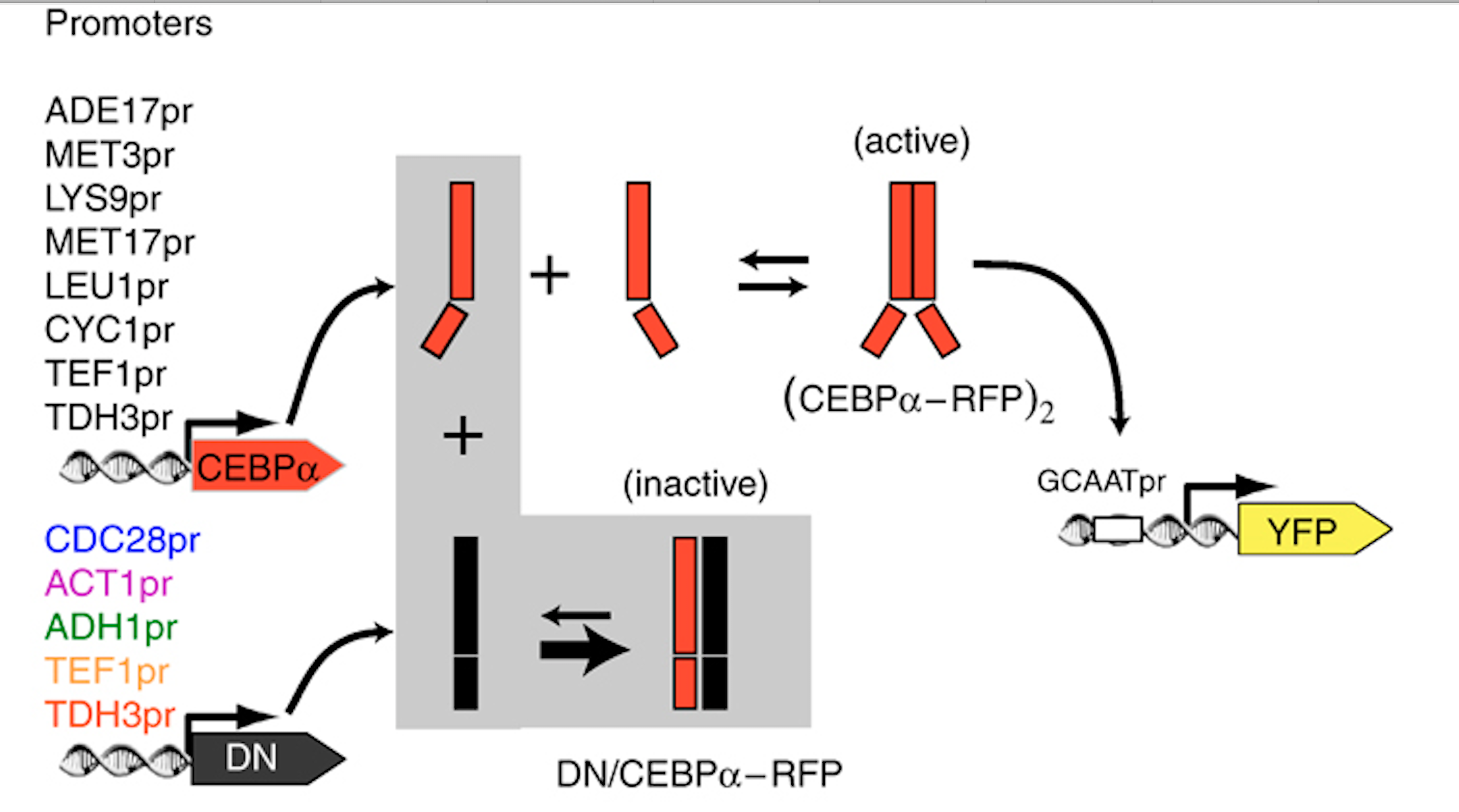
They engineered yeast cells to express a transcription factor, a stoichiometric inhibitor of that factor, and a target reporter gene to readout the level of the transcription factor. As an activator they used the mammalian bZip family activator CEBP/$\alpha$. As the inhibitor they used a previously identified dominant negative mutant that binds to CEBP/$\alpha$ with a tight $K_d \approx 0.04 nM$. As a reporter they used a yellow fluorescent protein. To vary the relative levels of the activator and inhibitor, they expressed them from promoters of different strengths. As a control, they also constructed yeast strains without the inhibitor.
The scheme is shown here:
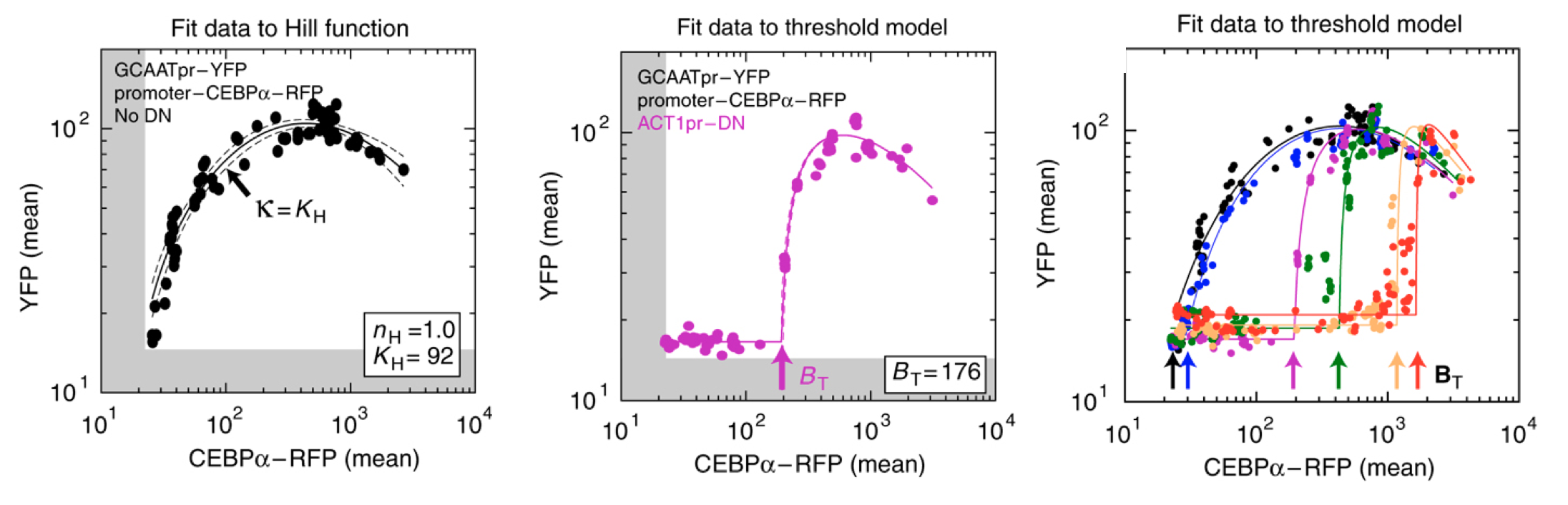
As shown below (left), the activator generated a dose-dependent increase in the fluorescent protein. (The noticeable decrease at the highest levels is attributed to the interesting effect of transcriptional "squelching"--see paper for details).
Adding the inhibitor (middle panel) produced the predicted threshold-linear response.
Finally, expressing the inhibitor from promoters of different strengths (right) showed corresponding shifts in the threshold position, as expected based on their independently measured expression levels (not shown).
The conclusions so far:
Tight binding can produce ultrasensitivity through molecular titration.
Molecular titration is a real effect that can be reconstituted and quantitatively predicted in living cells.
We now turn to biological contexts in which molecular titration appears.
small RNA regulation can generate ultrasensitive responses through molecular titration
One of the most stunning discoveries of the last several decades is the pervasive and diverse roles that small RNA molecules play in regulating gene expression, from bacteria to mammalian cells.
micro RNA (miRNA) represents a major class of regulatory RNA molecules in eukaryotes. Individual miRNAs typically target hundreds of genes. Conversely, most protein-coding genes are miRNA targets. miRNAs can be highly expressed (as much as 50,000 copies per cell).
Many miRNAs exhibit strong sequence conservation across species, suggesting selection for function.
However, at the cell population average level, they sometimes appear to generate relatively weak repression.
To more quantitatively understand how miRNA regulation operates, Mukherji et al developed a system to analyze miRNA regulation at the level of single cells (Mukherji, S., et al, Nat. Methods, 2011).
The key idea of the design is to express two distinguishable fluorescent proteins, one of which is regulated by a specific miRNA, with the other serving as an unregulated internal control.
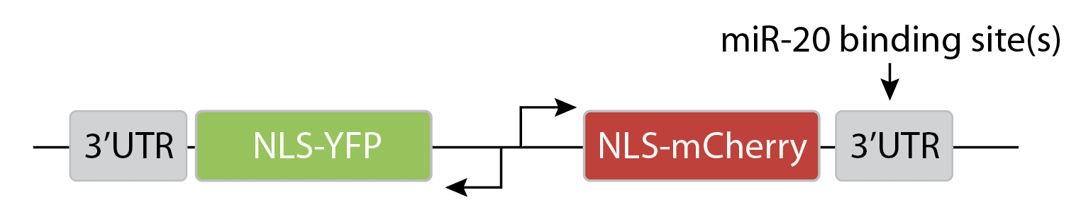
They transfected variants of this construct with (N=1) or without (N=0) a binding site for the miR-20 miRNA:
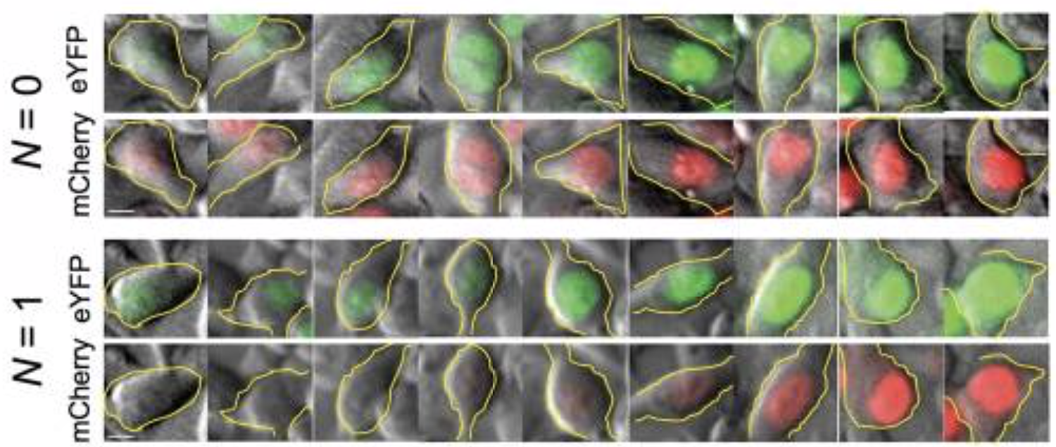
As you can see here, without the binding site, the two colors appear to be proportional to each other, as you would expect. But with the binding site, mCherry expression is differentially suppressed at lower YFP levels.
This can be seen more clearly in a scatter plot of the two colors:
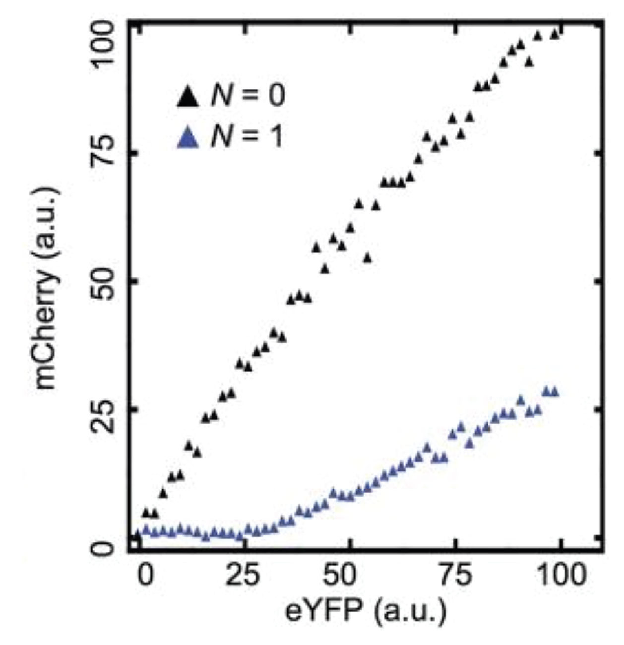
Here, the YFP x-axis is analogous to our $A_T$, above, while the mCherry y-axis is analogous to $A$.
The authors go on to explore how increasing the number of binding sites can modulate the threshold for repression. The results broadly fit the behavior expected from the molecular titration model.
These results could help reconcile the very different types of effects one sees for miRNAs in different contexts. Sometimes they appear to provide strong, switch-like effects, as with fate-controlling miRNAs in C. elegans. On the other hand, in many other contexts, they appear to exert much weaker "fine-tuning" effects on their targets. When miRNAs are unsaturated, they can have a relatively strong effect on their target expression levels, essentially keeping them "off." On the other hand, when targets are expressed highly enough, the relative effects of the miRNA on their expression can become much weaker.
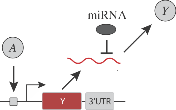
Returning to the question posed earlier, we now see that a remarkably simple way to create a threshold within a regulatory step is to insert a constitutive, inhibitory miRNA:
Note that in addition to its general regulatory abilities and thresholding effects, miRNA regulation can also reduce noise in target gene expression. See Schmiedel et al, "MicroRNA control of protein expression noise," Science (2015).
Molecular titration in antibiotic persistence
Antibiotic persistence is a phenomenon, which we already discussed, in which a small percentage of non-resistant cells survive antibiotic treatment. Once re-grown, the descendants of these cells behave the same as the original culture from which they were obtained, with the same small percentage surviving antibiotic treatment.
Nathalie Balaban and colleagues have used a variety of elegant approaches to analyze antibiotic persistence at the level of single cells. In Rotem et al, "Regulation of phenotypic variability by a threshold- based mechanism underlies bacterial persistence," PNAS (2010) they analyze the role of the hipAB toxin-antitoxin system in generating persisters.
The model for persistence described here combines three major concepts from the course so far: negative autoregulation, stochastic noise in gene expression, and, now, molecular titration.
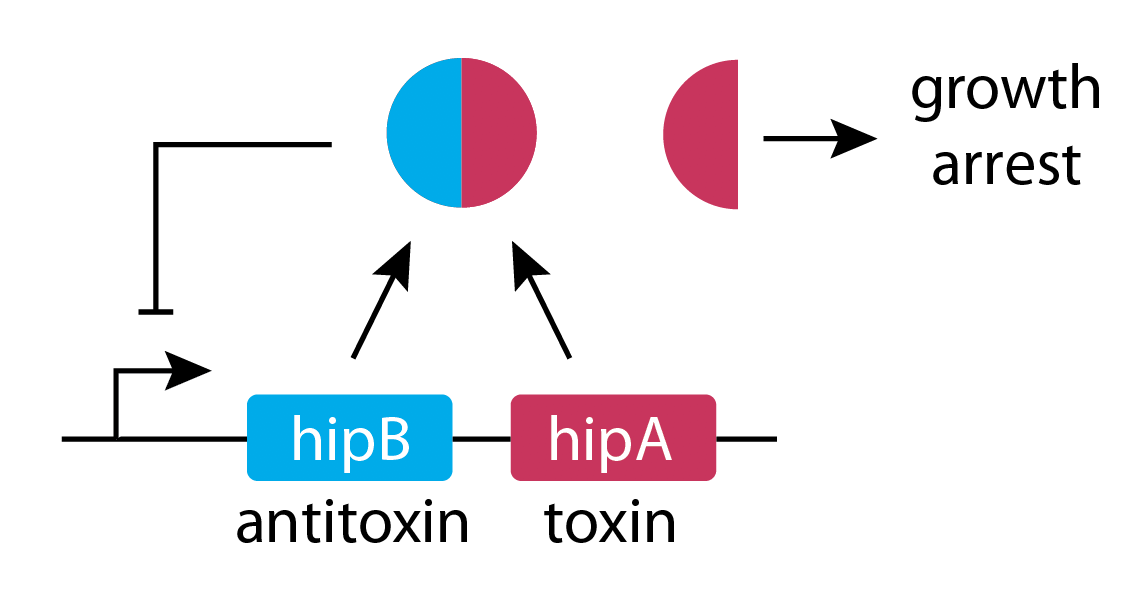
In this system, a protein "toxin", hipA, is neutralized by the anti-toxin hipB. The proteins are co-expressed in a single operon, and form a tight complex, which represses their own expression:
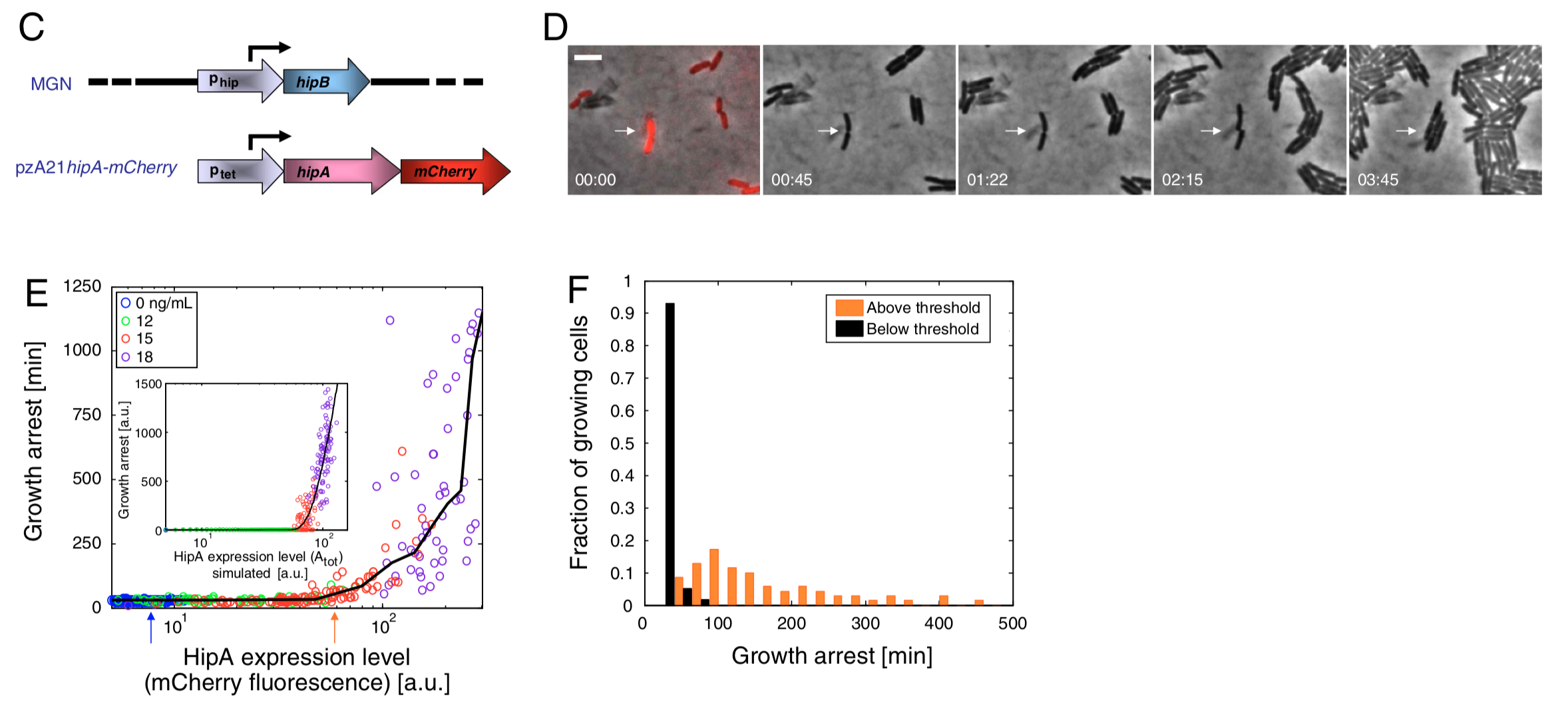
In a separate set of experiments, they tagged hipA with a red fluorecent protein, and used time-lapse movies to correlate the growth behavior of individual cells with their HipA protein levels.
As shown in these panels, there appeared to be a threshold relationship, in which growth arrest occurred when HipA (as measured by its fluorescent protein tag) exceeded a threshold concentration:
A simple model based on molecular titration, feedback, and noise can explain the key experimental features observed here. The model contains just a few reactions:
Production of HipA: $ P \rightarrow P+A $
Production of HipB: $ P \rightarrow P+B $
HipAB complex formation: $ A + B \leftrightarrow C $
Binding and unbinding of to DNA: $ P + C \leftrightarrow P_C $
Degradation and dilution of all protein species: $ A,B,C \rightarrow \emptyset $
Here $A$ and $B$ denote the HipA and HipB proteins, respectively, and $C$ represents the HipA-HipB complex. $P$ and $P_C$ represent the free and bound state of the hipAB promoter.
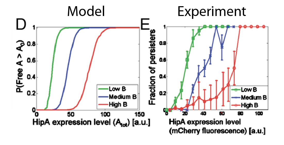
They simulated the model stochastically, with the assumption that free $A$ exceeding a threshold causes persistence. In this model, varying the expression level of the antitoxin, HipB, systematically shifted the threshold for persistence, a behavior that also occurred experimentally:
Beyond pairwise titration
Today we talked about molecular titration arising from interactions between protein pairs. However, proteins often form more complex, and even combinatorial, networks of homo- and hetero-dimerizing components. One example occurs in the control of cell death (apoptosis) by Bcl2-family proteins, a process that naturally should be performed in an all-or-none way. Another example that we will discuss soon involves the formation of signaling complexes in promiscuous ligand-receptor systems.
Conclusions
Today we have seen that molecular titration provides a simple but powerful way to generate ultrasensitive responses across different types of molecular systems:
The general principle of molecular titration: formation of a tight complex between two species makes the concentration of a "free" protein species depend in a threshold-linear manner on its total level or rate of production.
Molecular titration could explain key features of miRNA based regulation.
Molecular titration appears to underlie the generation of bacterial persisters through toxin-antitoxin systems.
Molecular titration between co-expressed, mutually inhibitory ligands and receptors can generate exclusive send-or-receive signaling states in the Notch signaling pathway.