22. Scaling reaction-diffusion patterns
(c) 2019 Justin Bois and Michael Elowitz. With the exception of pasted graphics, where the source is noted, this work is licensed under a Creative Commons Attribution License CC-BY 4.0. All code contained herein is licensed under an MIT license.
This document was prepared at Caltech with financial support from the Donna and Benjamin M. Rosen Bioengineering Center.

This lesson was generated from a Jupyter notebook. Click the links below for other versions of this lesson.
import numpy as np
import scipy.integrate

import biocircuits

import bokeh.layouts
import bokeh.plotting
import bokeh.io

bokeh.io.output_notebook()
Reaction-diffusion models for morphogen patterning
In the last lesson, we discussed morphogens, chemical species that determine cell fate in a concentration-dependent manner. Morphogens are spatially distributed throughout a developing organism, thereby imparting spatial variation in cell types. They present us with a great opportunity to connect our genetic network dynamics to spatial variation.
We specifically discussed two-component systems that give what is now known as Turing patterns. More generally, we can consider a set of biochemical species, $\mathbf{M} = \{M_1, M_2, \ldots\}$. The set of concentrations of these biochemical species is $\mathbf{c} = \{c_1, c_2, \ldots\}$. We can write down a system of partial differential equations describing the dynamics of morphogen concentrations (which is more or less a statement of conservation of mass) as
\begin{align} \frac{\partial c_i}{\partial t} &= \frac{\partial}{\partial x}\,D_i\,\frac{\partial c_i}{\partial x} + r_i(\mathbf{c}), \end{align}valid for all $i$. Here, $r_i(\mathbf{c})$ describes the net rate of production of species $M_i$, dependent on the concentrations of all other species. The diffusion coefficient $D_i$ parametrizes the diffusion of species $i$. For our purposes today, we are restricting ourselves to one-dimensional systems. We also have implicitly assumed that the diffusivity tensor is diagonal. Finally, for all of our analyses in this lecture, we will assume $x \in [0,L]$ with constant flux (usually no flux) boundary conditions at the ends of the domain. Recall that the flux of morphogen is given by Fick's first law,
\begin{align} j_i &= -D_i\,\frac{\partial c_i}{\partial x}. \end{align}A gradient from a point source
We will begin by analyzing the simplest case of morphogen patterning. We have a single morphogen, $M$, which has a source at $x = 0$. We model the source as a constant flux, $\eta$ at $x = 0$.
Simple decay of the morphogen
We begin with the case where our morphogen only undergoes a single reaction, degradation which we would represent as $M \to \emptyset$, and has a constant diffusion coefficient. Our PDE is
\begin{align} \frac{\partial c}{\partial t} &= D \,\frac{\partial^2 c}{\partial x^2} - \gamma c, \\[1em] \left.\frac{\partial c}{\partial x}\right|_{x=0} &= -\frac{\eta}{D}\\[1em] \left.\frac{\partial c}{\partial x}\right|_{x=L} &= 0. \end{align}We can readily solve for the unique steady state in this case as
\begin{align} c(x) = \frac{\eta}{\sqrt{D\gamma}}\,\frac{\mathrm{e}^{-x/\lambda} + \mathrm{e}^{(x-2L)/\lambda}}{1 - \mathrm{e}^{-2L/\lambda}}, \end{align}where $\lambda \equiv \sqrt{D/\gamma}$. So, we have an exponentially decaying morphogen profile with decay length $\lambda$. Typically, $L \gg \lambda$, so we have
\begin{align} c(x) &\approx \frac{\eta}{\sqrt{D\gamma}}\,\mathrm{e}^{-x/\lambda}. \end{align}Two obvious problems with this expression
Considering that morphogens determine cell fate in a concentration-dependent manner, there are two obvious problems with this expression.
- The total level of the morphogen is set by the strength of the source, $\eta$, assuming $D$ and $\gamma$ are constant. This would mean that cell fate would not be robust to the strength of the source.
- The decay length of the concentration profile is independent of size. This means that a larger organism would have all of its morphogen highly concentrated near $x/L = 0$.
Issue 2 is most clearly seen if we plot two profiles together.
# x-values for plot
L_1 = 100
L_2 = 200
x_1 = np.linspace(0, L_1, 200)
x_2 = np.linspace(0, L_2, 200)

# Value of lambda
lam = 25

# Make plots
p1 = bokeh.plotting.figure(height=250, width=350, x_axis_label='x/L', y_axis_label='conc')
p2 = bokeh.plotting.figure(height=250, width=350, x_axis_label='x/L', y_axis_type='log')
p1.line(x_1/L_1, np.exp(-x_1/lam), legend='L=100', line_width=2)
p1.line(x_2/L_2, np.exp(-x_2/lam), color='orange', legend='L=200', line_width=2)
p2.line(x_1/L_1, np.exp(-x_1/lam), line_width=2)
p2.line(x_2/L_2, np.exp(-x_2/lam), color='orange', line_width=2)

bokeh.io.show(bokeh.layouts.gridplot([[p1, p2]]))
We will address issue 1 in the homework. Now, we will consider a solution to issue 2 proposed by Ben-Zvi and Barkai (PNAS, 2010).
The concept of expansion repression
Consider another molecule, called an expander, that facilitates expansion of the morphogen. Specifically, the expander enhances diffusion of the morphogen and also prevents its degradation. However, and this is important because we need (you guessed it) feedback, the morphogen represses production of the expander. Our adjusted differential equations are now
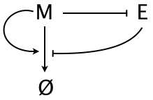
\begin{align} \frac{\partial c_m}{\partial t} &= \frac{\partial}{\partial x}\,D_m(c_m, c_e)\,\frac{\partial c_m}{\partial x} - \gamma_m(c_m, c_e)\, c_m \\[1em] \frac{\partial c_e}{\partial t} &= D_e \,\frac{\partial^2 c_e}{\partial x^2} + \frac{\beta_e}{1 + (c_m/k)^n} - \gamma_e\, c_e. \\ &\phantom{blah} \nonumber \end{align}We will consider the case where $D_m$ is constant, where the morphogen enhances its own degradation, and the expander represses degradation, shown schematically below.
The morphogen and expander are thus in a negative feedback loop. How might this help us with the issue that the morphogen gradient should scale? If we think about the construction of the gradient starting from no morphogen being present, the mechanism bcomes clear. Initially, we have no morphogen present, so the morphogen concentration grows throughout the entire tissue. As morphogen is introduced from the end of the tissue, the expander gets locally depleted. This leads to the morphogen spreading more toward the distal end of the tissue, where there is more expander, which inhibits the morphogen's degradation. However, as the morphogen levels toward the distal end rise, the expander can no longer limit the degradation of the morphogen because its production is inhibited by the elevated morphogen levels. Eventually, the expander level at the distal end is set by the balance of expander repression and morphogen degradation. This sets the level at the distal end, thereby setting the morphogen profile across the entire tissue.
In the absence of an expander, there is nothing to pin the value of the morphogen at the distal end, which means that the morphogen cannot "sense" how long the tissue is.
Numerical solution to R-D equations for simple degradation
We will first solve the system with simple degradation before treating the expander. To solve R-D systems, we can use the rd_solve() function from the biocircuits package. The function is general for 1D RD systems with a diagonal mobility tensor, but allows for nonconstant diffusion coefficients. We therefore need to provide the solver with a function to compute the reaction terms and the diffusion coefficients. For the oft used scenario where the diffusion coefficients are constant, we can use biocircuits.constant_diff_coeffs() for the latter.
We additionally need to provide the values of the derivatives at the boundaries to enforce the Neumann conditions. In this case, the flux is zero at the $x = L$ boundary, but given by $-\eta/\sqrt{D}$ at the $x = 0$ boundary to give the constant flux of morphogen.
def degradation_rxn(c_tuple, t, gamma):
    """
    Reaction expression for simple degradation.
    """
    return (-gamma * c_tuple[0],)

# Time points
t = np.linspace(0.0, 10.0, 100)

# Physical length of system
L = 5.0

# Diffusion coefficient
diff_coeffs = (1.0,)

# Gamma
rxn_params = (1.0,)

# Initial concentration (500 grid points)
c_0_tuple = (np.zeros(500), )

# Production rate
eta = 1.0
derivs_0 = -eta / np.sqrt(diff_coeffs[0])

# Solve
conc = biocircuits.rd_solve(c_0_tuple, t, L=L, derivs_0=derivs_0, derivs_L=0,
             diff_coeff_fun=biocircuits.constant_diff_coeffs,
             diff_coeff_params=(diff_coeffs,), rxn_fun=degradation_rxn,
             rxn_params=rxn_params)
And let's make a plot.
bokeh.io.show(biocircuits.rd_plot(conc, t, L))
Numerical solution of degradation with expander
To study the dynamics of the expander system, we will consider constant diffusion coefficients, and we take
\begin{align} \gamma_m(c_m, c_e) = (\gamma_{m,1} + \gamma_{m,2}c_m)\,\frac{c_m}{1+c_e}. \end{align}This means that in addition to natural degradation of the morphogen, we also have enhanced autodegradation, both of which are retarded by the expander. Thus, our PDEs are
\begin{align} \frac{\partial c_m}{\partial t} &= D_m \,\frac{\partial^2 c_m}{\partial x^2} - (\gamma_{m,1} + \gamma_{m,2}c_m)\,\frac{c_m}{1+c_e}, \\[1em] \frac{\partial c_e}{\partial t} &= D_e \,\frac{\partial^2 c_e}{\partial x^2} + \frac{\beta_e}{1 + (c_m/k)^n} - \gamma_e\, c_e. \end{align}Note the squared term in the degradation of the morphogen. This serves to make the gradient more robust to the source strength, as we will see in the homework.
We will perform the calculation for two values of $L$ and see how the gradient scales.
def expander_gradient_rxn(c_tuple, t, gamma_m1, gamma_m2, gamma_e,
                          beta_e, k, n):
    """
    Reaction expression for simple degradation.
    """
    # Unpack
    c_m, c_e = c_tuple

    # Morphogen reaction rate
    m_rate = -(gamma_m1 + gamma_m2 * c_m) * c_m / (1 + c_e)

    # Expander production rate
    e_rate = beta_e / (1 + (c_m / k)**n) - gamma_e * c_e

    return (m_rate, e_rate)

# Time points
t = np.linspace(0.0, 5e5, 300)

# Physical length of system and grid points
L_1 = 100.0
L_2 = 200.0
n_gridpoints = 100

# Diffusion coefficients
diff_coeffs = (1, 10)

# Reaction params
gamma_m1 = 0
gamma_m2 = 100
gamma_e = 1e-6
beta_e = 1e-2
k = 1e-3
n = 4
rxn_params = (gamma_m1, gamma_m2, gamma_e, beta_e, k, n)

# Initial concentration
c_0_tuple = (np.zeros(n_gridpoints), np.zeros(n_gridpoints))

# Production rate
eta = 10.0

# Solve
c_tuple_L_1 = biocircuits.rd_solve(
      c_0_tuple, t, L=L_1, derivs_0=(-eta, 0), derivs_L=0,
      diff_coeff_fun=biocircuits.constant_diff_coeffs, diff_coeff_params=(diff_coeffs,),
      rxn_fun=expander_gradient_rxn, rxn_params=rxn_params, atol=1e-7)

c_tuple_L_2 = biocircuits.rd_solve(
      c_0_tuple, t, L=L_2, derivs_0=(-eta, 0), derivs_L=0,
      diff_coeff_fun=biocircuits.constant_diff_coeffs, diff_coeff_params=(diff_coeffs,),
      rxn_fun=expander_gradient_rxn, rxn_params=rxn_params)
With the results in hand, we can compute the morphogen levels and see if we have scaling.
# x-values for plot
x_1 = np.linspace(0, L_1, n_gridpoints)
x_2 = np.linspace(0, L_2, n_gridpoints)

# Make plots
p1 = bokeh.plotting.figure(height=250, width=350, x_axis_label='x/L', y_axis_type='log')
p2 = bokeh.plotting.figure(height=250, width=350, x_axis_label='x', y_axis_type='log')
p1.line(x_1/L_1, c_tuple_L_1[0][-1,:], legend='L=100', line_width=2)
p1.line(x_2/L_2, c_tuple_L_2[0][-1,:], color='orange', legend='L=200', line_width=2)
p2.line(x_1, c_tuple_L_1[0][-1,:], line_width=2)
p2.line(x_2, c_tuple_L_2[0][-1,:], color='orange', line_width=2)

bokeh.io.show(bokeh.layouts.gridplot([[p1, p2]]));
Let's make a movie.
bokeh.io.show(biocircuits.rd_plot(c_tuple_L_1, t, L_1, normalize=True, legend_names=['morphogen', 'expander']))
Numerical solution for expander with non-cooperative degradation
We now consider the case where we do not have cooperative degradation. I.e., we have
\begin{align} \gamma_m(c_m, c_e) = \gamma_{m,1}\,\frac{c_m}{1+c_e}. \end{align}Thus, our PDEs are
\begin{align} \frac{\partial c_m}{\partial t} &= D_m \,\frac{\partial^2 c_m}{\partial x^2} - \gamma_{m,1}\frac{c_m}{1+c_e} \\[1em] \frac{\partial c_e}{\partial t} &= D_e \,\frac{\partial^2 c_e}{\partial x^2} + \frac{\beta_e}{1 + (c_m/k)^n} - \gamma_e\, c_e. \end{align}We can reuse the functions we already wrote with $\gamma_{m,1} >0$ and $\gamma_{m,2} = 0$.
# Reaction params
gamma_m1 = 0.1
gamma_m2 = 0
gamma_e = 1e-6
beta_e = 1e-2
k = 1e-3
n = 4
rxn_params = (gamma_m1, gamma_m2, gamma_e, beta_e, k, n)

# Initial concentration
c_0_tuple = (np.zeros(n_gridpoints), np.zeros(n_gridpoints))

# Production rate
eta = 0.1

# Solve
c_tuple_L_1 = biocircuits.rd_solve(
      c_0_tuple, t, L=L_1, derivs_0=(-eta, 0), derivs_L=0,
      diff_coeff_fun=biocircuits.constant_diff_coeffs, diff_coeff_params=(diff_coeffs,),
      rxn_fun=expander_gradient_rxn, rxn_params=rxn_params, atol=1e-6)

c_tuple_L_2 = biocircuits.rd_solve(
      c_0_tuple, t, L=L_2, derivs_0=(-eta, 0), derivs_L=0,
      diff_coeff_fun=biocircuits.constant_diff_coeffs, diff_coeff_params=(diff_coeffs,),
      rxn_fun=expander_gradient_rxn, rxn_params=rxn_params, atol=1e-6)

# x-values for plot
x_1 = np.linspace(0, L_1, n_gridpoints)
x_2 = np.linspace(0, L_2, n_gridpoints)

# Make plots
p1 = bokeh.plotting.figure(height=250, width=350, x_axis_label='x/L', y_axis_type='log')
p2 = bokeh.plotting.figure(height=250, width=350, x_axis_label='x', y_axis_type='log')
p1.line(x_1/L_1, c_tuple_L_1[0][-1,:], legend='L=100', line_width=2)
p1.line(x_2/L_2, c_tuple_L_2[0][-1,:], color='orange', legend='L=200', line_width=2)
p2.line(x_1, c_tuple_L_1[0][-1,:], line_width=2)
p2.line(x_2, c_tuple_L_2[0][-1,:], color='orange', line_width=2)

bokeh.io.show(bokeh.layouts.gridplot([[p1, p2]]));
Again, we get scaling of the gradient slope, but we see that the absolute level varies.