Homework 8
(c) 2019 Justin Bois and Michael Elowitz. With the exception of pasted graphics, where the source is noted, this work is licensed under a Creative Commons Attribution License CC-BY 4.0. All code contained herein is licensed under an MIT license.
This document was prepared at Caltech with financial support from the Donna and Benjamin M. Rosen Bioengineering Center.

This homework was generated from a Jupyter notebook. You can download the notebook here.
import numpy as np
8.1: Controlling p53 levels, 70 pts
p53 is an important protein for tumor suppression, DNA damage repair, cell cycle regulation, and more. In their 2012 paper, the researchers in Galit Lahav's group investigated how temporal dynamics of p53 controls cell fate in MCF-7 cells, a breast cancer cell line. It had been previously observed that p53 levels oscillate upon exposure to stress due to γ radiation. To instead study how cells respond to sustained levels of p53, the authors controlled p53 levels using the drug Nutlin-3. To do this, they devised a program for adjusting Nutlin-3 levels in the cell culture that would keep the p53 levels at a constant high level. They based this program on a mathematical model of the p53 circuit (shown in the figure below) that they developed and parametrized in an earlier paper.
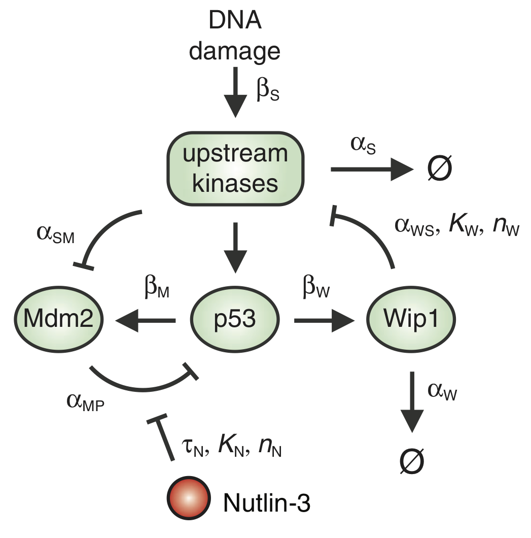
The p53 levels oscillate due to a delays in the autoinhibitory loops mediated by Mdm2 and Wip1. The dynamical equations for this circuit, as presented in the paper, are
\begin{align} \frac{\mathrm{d}P_i}{\mathrm{d}t} &= \beta_\mathrm{P} - \frac{\alpha_\mathrm{MP_i} \, M\,P_i}{1+\left(N(t-\tau_\mathrm{N})/K\right)^{n_\mathrm{N}}} - \beta_\mathrm{SP}\,P_i\,\frac{(S/T_\mathrm{S})^{n_\mathrm{S}}}{1 + (S/T_\mathrm{S})^{n_\mathrm{S}}} - \alpha_\mathrm{P_i}\, P_i,\\[1em] %% \frac{\mathrm{d}P_a}{\mathrm{d}t} &= \beta_\mathrm{SP}\,P_i\,\frac{(S/T_\mathrm{S})^{n_\mathrm{S}}}{1 + (S/T_\mathrm{S})^{n_\mathrm{S}}} - \frac{\alpha_\mathrm{MP_a} \, M\,P_a}{1+\left(N(t-\tau_\mathrm{N})/K\right)^{n_\mathrm{N}}},\\[1em] %% \frac{\mathrm{d}M}{\mathrm{d}t} &= \beta_\mathrm{M}\,P_a(t-\tau_\mathrm{M}) + \beta_{M_i} - \alpha_\mathrm{SM}\,S\,M - \alpha_M\,M,\\[1em] %% \frac{\mathrm{d}W}{\mathrm{d}t} &= \beta_\mathrm{W}\,P_a(t-\tau_\mathrm{W}) - \alpha_\mathrm{W}\,W,\\[1em] %% \frac{\mathrm{d}S}{\mathrm{d}t} &= \beta_\mathrm{S}\,\theta(t) - \alpha_\mathrm{WS}\,S\,\frac{(W/T_\mathrm{W})^{n_\mathrm{W}}}{1 + (W/T_\mathrm{W})^{n_\mathrm{W}}} - \alpha_\mathrm{S}\,S. \end{align}Here, $P_i$ and $P_a$ denote the concentrations of inactive and active p53, respectively. $M$ and $W$ are respectively the concentrations of Mdm2 and Wip1. The concentration of the DNA damage signal is denoted as $S$. Finally, $N$ is the externally imposed concentration of Nutlin-3. The function $\theta(t)$ is the Heaviside function. The parameters for the model are given in the code cell below. Before proceeding, take a moment and make sure you understand the physical meaning of each term in the equations.
# Parameters for p53 model
alpha_MPi = 5
alpha_Pi = 2
alpha_MPa = 1.4
alpha_SM = 0.5
alpha_M = 1
alpha_W = 0.7
alpha_WS = 50
alpha_S = 7.5
beta_P = 0.9
beta_SP = 10
beta_M = 0.9
beta_Mi = 0.2
beta_W = 0.25
beta_S = 10
tau_N = 0.4     # hours
tau_M = 0.7     # hours
tau_W = 1.25    # hours
K = 2.3         # µM
n_N = 3.3
n_S = 4
n_W = 4
T_W = 0.2
T_S = 1
a) Solve the equations numerically with $N = 0$. Plot the solution along with the experimental measurements from the Purvis, et al. paper, given in the Numpy arrays below. This helps verify that the model gives results similar to what you would observe experimentally.
# Time points (in units of hours)
time = np.array([0, 1, 2, 3, 4, 5, 6, 7, 8, 12])
relative_total_p53_conc = np.array([0.13, 0.69, 1.00, 0.87, 0.60,
                                    0.35, 0.34, 0.54, 0.61, 0.42])
b) Come up with a program for controlling the Nutlin-3 concentration so as to bring the total p53 level to a sustained value similar to that of its maximum value during oscillations in the absence of Nutlin-3. I.e., choose a function $N(t)$ to give a sustained level of p53 that is approximately unity (in the units specified by the parameter values). You might want to consider experimental constraints; for example that you might want to have only a few steps where the Nutlin-3 concentrations are adjusted to ease experimentation. Show a plot verifying that your scheme works.
8.2: Turing patterns with expanders (70 pts)
In this problem, we will explore scaling of Turing patterns, described by Werner, et al. (PRL, 2015). It will be helpful for you to refer to that paper in working this problem, but bear in mind that here we are using the same notation we have used throughout the course. I.e., $\gamma_A$ describes a degradation, as opposed to $\beta_A$ describing a degradation as it does in the paper.
As discussed in lecture, Turing patterns tend to have a wavelength that is independent of the size of the system, which means that they do not scale. Werner and coworkers propose a model for interactions of an expander with the classical Turing activator (A)-inhibitor (B) components. This model is shown in Fig. 3a of the paper.
a) The authors use the following set of PDEs for the Turing system without the expander.
\begin{align} \frac{\partial a}{\partial t} &= D_A\,\frac{\partial^2 a}{\partial x^2} + \beta_A\,\frac{a^n}{a^n + b^n} - \gamma_A a \\[1em] \frac{\partial b}{\partial t} &= D_B\,\frac{\partial^2 b}{\partial x^2} + \beta_B\,\frac{a^n}{a^n + b^n} - \gamma_B b. \end{align}- They seem to have chosen a peculiar functional form for the mutual regulation of A and B, $a^n/(a^n + b^n)$. Describe in words how this captures the components of the diagram for the Turing system (inside the dotted box of Fig. 3a of the paper).
- Show that we can nondimensionalize this system to be
where $a$, $b$, $x$, and $t$ are now dimensionless. Importantly, $x$ has been nondimensionalized with the characteristic length scale $\lambda_A = \sqrt{D_A/\gamma_A}$.
- Find the unique homogeneous steady state of this system. By homogeneous steady state, we mean that the concentration profiles of $a$ and $b$ are uniform in space and the time derivatives vanish.
- Starting from a small perturbation of this steady state, numerically solve the coupled PDEs. Use no-flux boundary conditions. Plot the resulting steady state concentration profiles for $a$ and $b$. Do this using the following parameters: $d_b = 30$, $\beta_b = 4$, $\gamma_b = 2$, and $n = 5$. Do this five times, once each for the total dimensionless length of the system being 5, 10, 20, 40, and 80. Comment on the pertinence of these results with respect to scaling.
b) We will now consider the system in the presence of an expander, E. The new dimensional equations are
\begin{align} \frac{\partial a}{\partial t} &= D_A\,\frac{\partial^2 a}{\partial x^2} + \beta_A\,\frac{a^n}{a^n + b^n} - \kappa_A e a \\[1em] \frac{\partial b}{\partial t} &= D_B\,\frac{\partial^2 b}{\partial x^2} + \beta_B\,\frac{a^n}{a^n + b^n} - \kappa_B e b\\[1em] \frac{\partial e}{\partial t} &= D_E\,\frac{\partial^2 e}{\partial x^2} + \beta_E - \kappa_E e b. \end{align}- Give a brief description on how this relates to the schematic in Fig. 3a of the Werner, et al. paper) and comment on any approximations that are being made.
- Show that these equations may be nondimensionalized to read
Importantly, note that this nondimensionalization has a different length scale than the original system. We now have $\lambda_0 = \sqrt{D_A/\sqrt{\kappa_A \beta_A}}$.
- There is no homogeneous steady state for this system. For our initial "steady state" when doing the numerical calculations in part (iv), we will take $e_0 = 1$ and solve for the values of $a$ and $b$ such that $\mathrm{d}a/\mathrm{d}t = \mathrm{d}b/\mathrm{d}t = 0$. Nevermind that for this "steady state," $\mathrm{d}e/\mathrm{d}t \ne 0$.
- Again, starting from a small perturbation of this "steady state," numerically solve the coupled PDEs using no-flux boundary conditions. Plot the resulting steady state concentration profiles for $a$ and $b$. Do this using the same parameters as in part (a-4), with additional parameters $d_e = 10$, $\beta_e = 0.4$, $\kappa_b = 2$, and $\kappa_e = 2$. Again, do this five times, once each for the total dimensionless length of the system being 5, 10, 20, 40, and 80. (You can do it for more lengths if you like.) Comment on the pertinence of these results with respect to scaling.
c) Comment qualitatively on how the expander works to scale the Turing patterns. By what other means (other than mutual inhibition of B and inhibition of A) might an expander operate? Remember, these models are postulates of what might be happening in developing organisms, so it is useful to dream up alternatives.
8.3: Feedback on the course, 30 pts
We are always looking to improve the course, so we solicit feedback from students at the end. We are also planning on putting out our Jupyter notebooks (heavily edited, since you were working with a first draft this term) for the world to use. We greatly appreciate your thoughtful comments. Please submit the results of this problem both as text in the body of your email submission and within your submitted notebook. Thank you for doing this, and thank you also for a great term!
Notebooks and their structure
- What would you add/delete/change to the lesson notebooks to make them most useful both for the course itself and as an enduring resource for future research and learning?
- Did you like how the techniques and concepts were integrated together in the notebooks, or would you prefer to have these things separated? (One possibility is to have an appendix to the notebooks that serves as a reference for the techniques used in the course.)
- Was the biocircuits package useful? Do you have any suggestions for improving it?
- Do you have any suggestions for notebook organization?
Content
- What biological topics did you find most or least interesting, and why?
- What methods and approaches required more (or less) depth?
- How was the balance of conceptual / analytical / computational approaches?
- Which homework problems were most valuable?
- We are considering having original data from the papers we study in our lessons incorporated into the notebook and demonstrate how we can draw the conclusions of the papers from the data. The idea is that this will bring in an important skill set to a researcher who wants to work with biological circuits, but our concern is clutter.
Any other suggestions?
- Any other thoughts or comments appreciated.