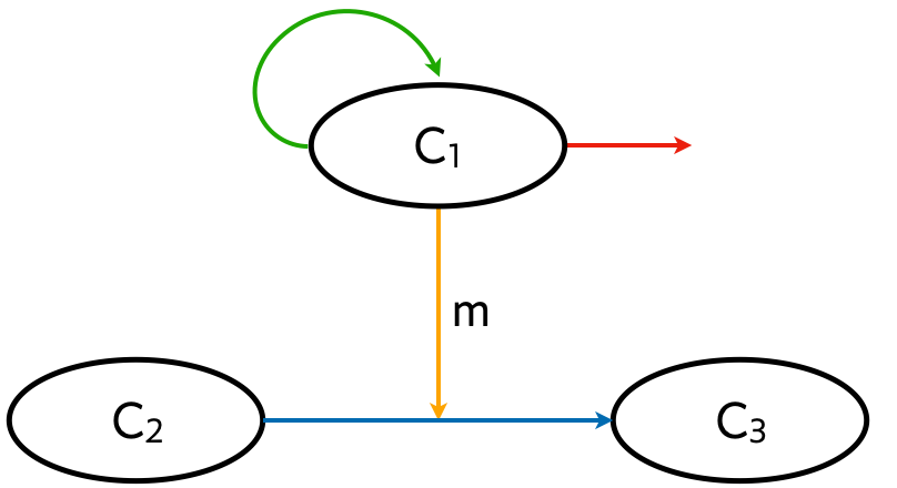
We have mostly been considering circuits of genes and their products within single cells. Like genes, cells can form circuits, called cellular circuits. A cellular circuit can involve four main types of interactions, depicted in the example circuit below.

- Proliferation (green arrow).
- Secretion (orange arrow).
- Differentiation (blue arrow).
- Cell death (red arrow).
In the example circuit, the secreted molecule m affects differentiation of cells of type 2 into those of type 3, but a secreted molecule in general may have any arbitrary effect on cellular behavior.
An important feature of cellular circuits is that they are necessarily autocatalytic in that cells are necessary to proliferate. While the simplest model for gene expression, that of unregulated expression, was
\begin{align} \frac{\mathrm{d}x}{\mathrm{d}t} = \beta - \gamma x, \end{align}where $x$ is the concentration of the gene product, the simplest model for a cellular circuit, that of unregulated division and cell death has a different form,
\begin{align} \frac{\mathrm{d}x}{\mathrm{d}t} = \beta x - \gamma x, \end{align}where $x$ here is the concentration of cells. Note that the production term is linear in $x$. There is only one steady state for this system, $x = 0$. If $\gamma > \beta$, the steady state is stable; the cells die out more rapidly than they can divide. However, if $\beta > \gamma$, the cells grow without bound. Physically, $then, \beta$ is a function of $x$ as well, and saturates for large $x$. In practice, there are many regulatory processes governing cell growth, and also death, and this leads to more stable nonzero steady states and interesting dynamics.
Cellular circuits abound, both in single-cell and multicellular organisms. In this problem we will analyze a cellular circuit featuring biphasic control of cell populations, in which a molecule is favorable for cell growth at moderate concentrations, but detrimental if in very small or very large concentrations.
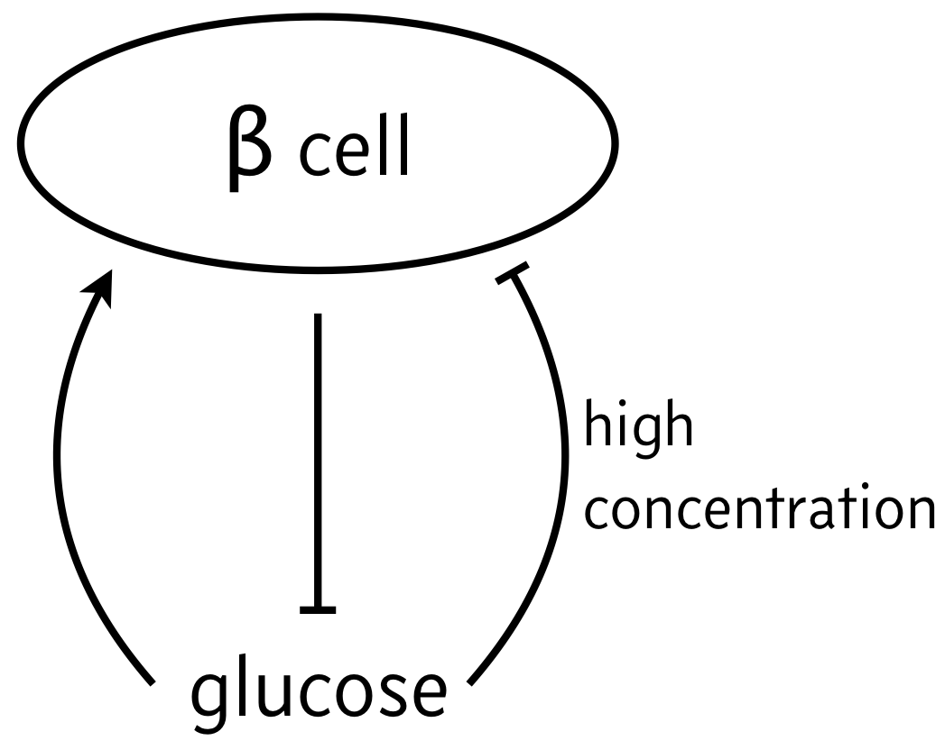
As a classic example of biphasic control, we can think of the relationship between β cells and glucose. In response to elevated glucose levels, β cells secrete insulin, which serves to reduce glucose levels. But if glucose levels get too high, it is toxic to the β cells, which can then die off. So, the propensity for β cells to produce insulin (simply noted "β cells" in the schematic below) is maximal at intermediate levels of glucose.

We will investigate the consequences of this circuit architecture in this problem. In doing so, we will review many of the important techniques from dynamical systems in analyzing biological circuits. The analysis we will do closely follows Karin and Alon, Molec. Sys. Biol., 2017.
We model the cellular circuit with a system of ODEs as follows.
\begin{align} \frac{\mathrm{d}c}{\mathrm{d}t} &= (\beta_c(m) - \gamma_c(m))\,c \\[1em] \frac{\mathrm{d}m}{\mathrm{d}t} &= \beta_m - \gamma_m(c)\,m. \end{align}The production and degradation rate of insulin producing β cells are both dependent on the glucose concentration $m$ and are proportional to the cell concentration $c$. The parameter $\beta_m$ is the feed rate of glucose, which is accomplished in an organism by eating and drinking, or in a cell culture by injection of glucose.
We choose the following forms for the functions above.
\begin{align} \beta_c(m) &= \beta_{c,1}\,\frac{(m/k_\beta)^{n_\beta}}{1 + (m/k_\beta)^{n_\beta}},\\[1em] \gamma_c(m) &= \gamma_{c,0} + \gamma_{c,1}\,\frac{(m/k_\gamma)^{n_\gamma}}{1 + (m/k_\gamma)^{n_\gamma}}, \\[1em] \gamma_m(c) &= \gamma_{m,1}\,c. \end{align}a) Describe in words what the respective terms in these expressions mean.
b) Nondimensionalize the dynamical equations to give
\begin{align} \frac{\mathrm{d}c}{\mathrm{d}t} & = \left(\beta_c\,\frac{m^{n_\beta}}{1 + m^{n_\beta}} - 1 - \gamma\,\frac{(\kappa m)^{n_\gamma}}{1 + (\kappa m)^{n_\gamma}}\right)c, \\[1em] \frac{\mathrm{d}m}{\mathrm{d}t} &= \beta_m - cm. \end{align}c) In our numerical analysis, we will use the parameters from the Karin and Alon paper,
\begin{align} &\beta_m = 3.79 \\[1em] &\beta_c = 16.0 \\[1em] &\gamma = 20.0 \\[1em] &\kappa = 0.875 \\[1em] &n_\beta = 6 \\[1em] &n_\gamma = 6. \end{align}Numerically solve the dimensionless dynamical equations, once for an initial condition with low cell density ($c(0) = 2$) and again for an initial condition with high cell density ($c(0) = 5$). In both cases, take the initial glucose concentration to be $m(0) = 1/2$.
At low initial β cell density, you will see that the cells stop producing insulin and the glucose concentration grows to high levels, a "diabetes condition." Conversely, when the number of β cells producing insulin is higher (dashed lines), they stabilize and maintain a consistent insulin level.
d) To get a more complete graphical picture of the dynamics, your task is to build a phase portrait. The plot should include all nullclines, fixed points (open circle for unstable, closed for stable), separatrices, and the phase portrait (flow field).
i) The $c$-nullcline is the set of values of $m$ and $c$ for which $\mathrm{d}c/\mathrm{d}t = 0$. Show that $c = 0$ is part of the $c$-nullcline.
ii) To complete the $c$-nullcline, show analytically that there can be zero, one, or two values of $m$ for which $\mathrm{d}c/\mathrm{d}t = 0$, regardless the value of $c$. For the parameters above, solve numerically for these values of $m$. Hint: There will be two of them.
iii) Write an expression for the $m$-nullcline. That is the nullcline defined by $\mathrm{d}m/\mathrm{d}t = 0$. Using this result, and the one from part (i), show that $c = 0, \; m\to\infty$ is a fixed point. This is the diabetes condition. Obviously, you cannot display this fixed point on your plot.
iv) Perform a stability analysis about each of the fixed points you found.
v) Plot the nullclines and the fixed points, except for the one at $m\to\infty$.
vi) In looking at your numerical solutions from part (c), if we start with $c = 2$ and $m = 1/2$, the system carries us away toward the diabetic state with runaway glucose and no β cells producing insulin. Conversely, if we start with $c=5$ and $m=1/2$, the system progresses toward the stable fixed point. In moving from $c = 2$ to $c = 5$, we have crossed a separatrix in $c$-$m$ space. The qualitative behavior of the system changes by crossing that line.
The separatrix goes through the unstable fixed point which is a saddle. A saddle has one positive eigenvalue, but the other eigenvalues are negative. The system is thus attracted to the saddle fixed point along the eigenvector corresponding to the negative eigenvalues, before pushing away from the fixed point along the eigenvector corresponding to the positive eigenvalue.
To plot the separatrix, we can start at the unstable fixed point, and then take a tiny step along the eigenvector corresponding to the negative eigenvalue. We will call this eigenvector $\mathbf{v}$. We then integrate the dynamical system backwards in time to generate the separatrix. This enables us to trace out the path that attracts the system toward the saddle. We can do the same thing stepping just off of the saddle fixed point in the $-\mathbf{v}$ direction. This enables use to plot a separatrix separating dynamics that go right toward the stable fixed point or left toward runaway glucose. Add the separatrix to your plot. (There is only one, as there is only one unstable fixed point.)
vii) Finally, overlay the phase portrait. Based on this graphical analyses, comment on the importance of having high β cell levels.