5. Analysis of feed forward loops

---

Design principles

• The C1-FFL with AND logic has an on-delay, but no off-delay.

• The C1-FFL with OR logic has an off-delay, but no on-delay.

• The C1-FFL with both AND and OR logic can filter out short input impulses.

• The I1-FFL with AND logic is a pulse generator and also speeds response compared to an unregulated circuit.

Concept

• When multiple factors regulate a single gene, we need to specify the logic of the regulation, usually OR or AND.

---

import numpy as np
import scipy.integrate

import biocircuits

import bokeh.io
import bokeh.plotting

import colorcet

import panel as pn

bokeh.io.output_notebook()
pn.extension()

colors = colorcet.b_glasbey_category10

Loading BokehJS ...

---

In this lesson, we will discuss the feed forward loop, or FFL. We discovered in the previous lesson that this is a prevalent motif in E. coli. That is to say that the FFL appears more often, in fact much more often, in circuits present in E. coli that would be expected by random chance. Given the prevalence of FFLs, they most likely are doing something. To get to the bottom of this, we will do a full analysis of them in this lecture.

Categorizing FFLs

The architecture of the FFL was discussed in the last lecture. It consists of three genes, which we will call X, Y, and Z. We think of X as an input that regulates both Y and Z. Y regulates Z. The regulation can be either activating or repressing (or something more complicated, but we will restrict our attention to these two). So, there are three interactions to consider, X’s regulation of Y, X’s regulation of Z, and Y’s regulation of Z. There are two choices of mode of regulation for each, so there are a total of \(2^3 = 8\) different FFLs. These are shown below, in a figure taken from Alon, Nature Rev. Genet., 2007. Abbreviations for these circuits are commonly used. E.g., C2-FFL is the coherent FFL of type 2 and I4-FFL is the incoherent FFL of type 4.

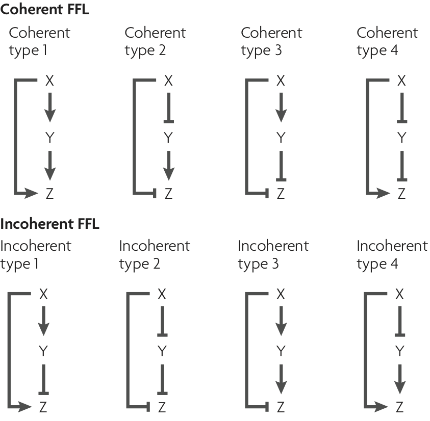
Half of the FFL architectures are coherent and half are incoherent. For those that are coherent, X’s direct regulation of Z and its indirect regulation of Z are the same, either both activating or both repressing. For incoherent FFLs, X’s direct and indirect regulation are not the same.

The most-encountered FFLs

While FFLs in general are motifs, some FFLS are more often encountered than others. In the figure below, also taken from the Alon review, we see relative abundance of the eight different FFLs in E. coli and S. cerevisiae. Two FFLs, C1-FFL and I1-FFL stand out as having much higher abundance than the other six.

We will take a look at these two FFLs in turn to see what features they might provide. First, though, we need to consider the logic of regulation by more than one transcription factor.

Logic of regulation by two transcription factors

Because X and Y both regulate Z in an FFL, we need to specify how they do that.

For the sake of illustration, let us assume we are discussing C1-FFL, where X activates Z and Y also activates Z. One can imagine a scenario where both X and Y need to be present to turn on Z. For example, they could be binding partners that together serve to recruit polymerase to the promoter. We call this AND logic. In other words, to get expression of Z, we must have X AND Y. Conversely, if either X or Y may each alone activate Z, we have OR logic. That is, to get expression of Z, we must have X OR Y.

So, to fully specify an FFL, we need to also specify the logic of how Z is regulated. So, we might have, for example, a C1-FFL with OR logic. This gives a total of 16 possible FFLs.

We are now left with the task of figuring out how to encode AND and OR logic.

Logic with two activators

Let us start first with Y and Z both activating with AND logic. We can construct a truth table for whether or not Z is on, given the on/off status of X and Y. The truth table is shown below, with a zero entry meaning that the gene is not on and a one entry meaning it is on.

X	Y	Z
0	0	0
0	1	0
1	0	0
1	1	1

We can also construct a truth table for OR logic with X and Y both activating.

X	Y	Z
0	0	0
0	1	1
1	0	1
1	1	1

The dynamics of the concentration of Z may be written as

\begin{align} \frac{\mathrm{d}z}{\mathrm{d}t} = \beta_0\,f(x, y) - \gamma z. \end{align}

Our goal is to specify the dimensionless function \(f(x, y)\) that encodes the appropriate truth table. How do we encode it with Hill functions? We could derive the functional form from the molecular details of the promoter region and the activators. Instead, we will again use a phenomenological Hill function. (Again, we could show that these Hill functions match certain promoter architectures.) The following functions work.

\begin{align} &\text{AND logic: } f(x,y) = \frac{(x/k_x)^{n_x} (y/k_y)^{n_y}}{1 + (x/k_x)^{n_x} (y/k_y)^{n_y}},\\[1em] &\text{OR logic: } f(x,y) = \frac{(x/k_x)^{n_x} + (y/k_y)^{n_y}}{1 + (x/k_x)^{n_x} + (y/k_y)^{n_y}}. \end{align}

In what follows, we will take \(x/k_x \to x\) and \(y/k_y \to y\) such that \(x\) and \(y\) are now dimensionless, nondimensionalized by their Hill \(k\). In this notation, we have

\begin{align} &\text{AND logic: } f(x,y) = \frac{x^{n_x} y^{n_y}}{1 + x^{n_x} y^{n_y}},\\[1em] &\text{OR logic: } f(x,y) = \frac{x^{n_x} + y^{n_y}}{1 + x^{n_x} + y^{n_y}}. \end{align}

We can make plots of these functions to demonstrate how they represent the respective logic.

def contourf(x, y, z, title=None, palette="Viridis256"):
    """Make a filled contour plot given x, y, z data given in 2D arrays."""
    p = bokeh.plotting.figure(
        frame_height=200,
        frame_width=200,
        x_range=(x.min(), x.max()),
        y_range=(y.min(), y.max()),
        x_axis_label="x",
        y_axis_label="y",
        title=title,
    )
    p.image(
        image=[z],
        x=x.min(),
        y=y.min(),
        dw=x.max() - x.min(),
        dh=x.max() - x.min(),
        palette=palette,
        alpha=0.8,
    )

    return p


# Get x and y values for plotting
x = np.linspace(0, 2, 200)
y = np.linspace(0, 2, 200)
xx, yy = np.meshgrid(x, y)

# Parameters (steep Hill functions)
nx = 20
ny = 20

# Regulation functions
def aa_and(x, y, nx, ny):
    return x ** nx * y ** ny / (1 + x ** nx * y ** ny)


def aa_or(x, y, nx, ny):
    return (x ** nx + y ** ny) / (1 + x ** nx + y ** ny)


# Generate plots
plots = [
    contourf(
        xx, yy, aa_and(xx, yy, nx, ny), title="two activators, AND logic"
    ),
    contourf(xx, yy, aa_or(xx, yy, nx, ny), title="two activators, OR logic"),
]

bokeh.io.show(bokeh.layouts.row(plots))

Here, purple indicates that \(f(x, y)\) is zero and yellow indicates that \(f(x, y)\) is one. With AND logic, both X and Y must have high concentrations for Z to be expressed. Conversely, for OR logic, either X or Y can be in high concentrations for Z to be expressed, but if neither is high enough, Z does not get expressed. The equations phenomenologically capture the logic.

Logic with two repressors

Now let’s consider the case where we have two repressors, as in the C3-FFL or I2-FFL. The AND case where X and Y are both repressors is NOT X AND NOT Y. This is equivalent to a NAND gate, with the following truth table.

X	Y	Z
0	0	1
0	1	1
1	0	1
1	1	0

We might get this kind of logic if the two repressors need to work in concert, perhaps through binding interactions, to affect repression.

For OR logic with two repressors, we have NOT X OR NOT Y, which is a NOR gate. Its truth table is below.

X	Y	Z
0	0	1
0	1	0
1	0	0
1	1	0

Here, either repressor (or both) can shut down gene expression.

We can encode these two truth tables with dimensionless regulation functions

\begin{align} &\text{AND logic: } f(x,y) = \frac{1}{(1 + x^{n_x}) (1 + y^{n_y})},\\[1em] &\text{OR logic: } f(x,y) = \frac{1 + x^{n_x} + y^{n_y}}{(1 + x^{n_x}) ( 1 + y^{n_y})}. \end{align}

Let’s make some plots to see how these functions look.

# Regulation functions
def rr_and(x, y, nx, ny):
    return 1 / (1 + x ** nx) / (1 + y ** ny)


def rr_or(x, y, nx, ny):
    return (1 + x ** nx + y ** ny) / (1 + x ** nx) / (1 + y ** ny)


# Generate plots
plots = [
    contourf(xx, yy, rr_and(xx, yy, nx, ny), title="two repressors, AND logic"),
    contourf(xx, yy, rr_or(xx, yy, nx, ny), title="two repressors, OR logic"),
]

bokeh.io.show(bokeh.layouts.row(plots))

Logic with one activator and one repressor

Now say we have one activator (which we will designate to be X) and one repressor (which we will designate to be Y). Now, AND logic means X AND NOT Y, and OR logic means X OR NOT Y. The truth table for the AND gate is below.

X	Y	Z
0	0	0
0	1	0
1	0	1
1	1	0

And that for the OR gate is

X	Y	Z
0	0	1
0	1	0
1	0	1
1	1	1

The dimensionless regulatory functions are

\begin{align} &\text{AND logic: } f(x,y) = \frac{x^{n_x}}{1 + x^{n_x} + y^{n_y}},\\[1em] &\text{OR logic: } f(x,y) = \frac{1 + x^{n_x}}{1 + x^{n_x} + y^{n_y}}. \end{align}

Finally, let’s look at a plot.

# Regulation functions
def ar_and(x, y, nx, ny):
    return x ** nx / (1 + x ** nx + y ** ny)


def ar_or(x, y, nx, ny):
    return (1 + x ** nx) / (1 + x ** nx + y ** ny)


# Generate plots
plots = [
    contourf(
        xx,
        yy,
        ar_and(xx, yy, nx, ny),
        title="X activates, Y represses, AND logic",
    ),
    contourf(
        xx,
        yy,
        ar_or(xx, yy, nx, ny),
        title="X activates, Y represses, OR logic",
    ),
]

bokeh.io.show(bokeh.layouts.row(plots))

For both kinds of logic, gene expression is on if Y is not too high relative to X. In the case of AND logic, X also much be sufficiently high.

Dynamical equations for FFLs

To analyze the C1-FFL and I1-FFL (or any of the other FFLs), in response to changes in the input X, we can write a generic system of ODEs for the concentrations of Y and Z. We know that Y is either activated or repressed by X and itself experiences degradation. We define a dimensionless function \(f_y(x/k_{xy}; n_{xy})\) to describe the activating or repressive Hill function for the regulation of X by Y. We have used the notation that \(n_{ij}\) is the Hill coefficient for j regulated by i, with \(k_{ij}\) similarly defined. To be explicit, if X activates Y, then

\begin{align} f_y(x/k_{xy}; n_{xy}) = \frac{(x/k_{xy})^{n_{xy}}}{1 + (x/k_{xy})^{n_{xy}}}, \end{align}

and if X represses Y, then

\begin{align} f_y(x/k_{xy}; n_{xy}) = \frac{1}{1 + (x/k_{xy})^{n_{xy}}}. \end{align}

The dynamical equation for \(y\) for either activating or repressive action by X is

\begin{align} \frac{\mathrm{d}y}{\mathrm{d}t} &= \beta_y\,f_y(x/k_{xy}; n_{xy}) - \gamma_y y. \end{align}

Similarly, we define the dimensionless function \(f_z(x/k_{xz}, y/k_{yz}; n_{xz}, n_{yz})\) to describe the regulation in expression of Z by X and Y. This have any of the functional forms we have listed above for activation/repression pairs and AND/OR logic. The dynamical equation for \(z\) is then

\begin{align} \frac{\mathrm{d}z}{\mathrm{d}t} &= \beta_z\,f_z(x/k_{xz}, y/k_{yz}; n_{xz}, n_{yz}) - \gamma_z z. \end{align}

We can nondimensionalize these equations by choosing

\begin{align} t &= \tilde{t} / \gamma_y, \\[1em] x &= k_{xz}\,\tilde{x},\\[1em] y &= k_{yz}\,\tilde{y},\\[1em] z &=z_0\,\tilde{z}, \end{align}

where \(z_0\) is as of yet unspecified. Inserting these expressions into the dynamical equations gives

\begin{align} \gamma_y k_{yz}\,\frac{\mathrm{d}\tilde{y}}{\mathrm{d}\tilde{t}} &= \beta_y\,f_y\left(\frac{k_{xz}}{k_{xy}}\,\tilde{x}; n_{xy}\right) - \gamma_y k_{yz} \tilde{y},\\[1em] \gamma_y z_0\,\frac{\mathrm{d}\tilde{z}}{\mathrm{d}\tilde{t}} &= \beta_z\,f_z(\tilde{x}, \tilde{y}; n_{xz}, n_{yz}) - \gamma_z z_0 \tilde{z}. \end{align}

If we conveniently define \(z_0 = \beta_z/\gamma_z\), then the dynamical equations become

\begin{align} \frac{\mathrm{d}\tilde{y}}{\mathrm{d}\tilde{t}} &= \beta\,f_y\left(\kappa\tilde{x}; n_{xy}\right) - \tilde{y},\\[1em] \gamma^{-1}\,\frac{\mathrm{d}\tilde{z}}{\mathrm{d}\tilde{t}} &= f_z(\tilde{x}, \tilde{y}; n_{xz}, n_{yz}) - \tilde{z}, \end{align}

where we have defined

\begin{align} &\beta = \frac{\beta_y}{\gamma_y k_{yz}},\\[1em] &\gamma = \frac{\gamma_z}{\gamma_y}, \\[1em] &\kappa = \frac{k_{xz}}{k_{xy}}. \end{align}

In addition to the Hill coefficients, these dimensionless parameters complete the parameter set of the FFL dynamical system. Each has a physical meaning. The parameter \(\beta\) is the dimensionless unregulated steady state level of \(y\), \(\gamma\) is the ratio of the decay rates of Z and Y, and \(\kappa\) is the ratio of the amounts of X that are necessary to regulate Z and Y.

Henceforth, we will work with these dimensionless equation and will drop the tildes for notational convenience.

Numerical solution of the FFL circuits

To specify the dynamical equations so that we may numerically solve them, we need to specify the functions \(f_y\) and \(f_z\) along with their Hill coefficients. The function \(f_y\) is either an activating or repressive Hill function, and the functions \(f_z\) have already been defined as aa_and(), aa_or(), etc., above. For convenience in future lessons, these functions are included in the biocircuits.reg submodule.

Let’s proceed to code up the right-hand side of the dynamical equations for FFLs. It is convenient to define a function that will give back a function that we can use as the right-hand side we need to specify to scipy.integrate.odeint(). Remember that odeint() requires a function of the form func(yz, t, *args), where yz is an array of length containing the values of \(y\) and \(z\). For convenience, our function will return a function with call signature rhs(yz, t, x), where x is the value of \(x\) at a given time point.

def ffl_rhs(beta, gamma, kappa, n_xy, n_xz, n_yz, ffl, logic):
    """Return a function with call signature fun(yz, x) that computes
    the right-hand side of the dynamical system for an FFL. Here,
    `yz` is a length two array containing concentrations of Y and Z.
    """
    if ffl[:2].lower() in ("c1", "c3", "i1", "i3"):
        fy = lambda x: biocircuits.reg.act_hill(x, n_xy)
    else:
        fy = lambda x: biocircuits.reg.rep_hill(x, n_xy)

    if ffl[:2].lower() in ("c1", "i4"):
        if logic.lower() == "and":
            fz = lambda x, y: biocircuits.reg.aa_and(x, y, n_xz, n_yz)
        else:
            fz = lambda x, y: biocircuits.reg.aa_or(x, y, n_xz, n_yz)
    elif ffl[:2].lower() in ("c4", "i1"):
        if logic.lower() == "and":
            fz = lambda x, y: biocircuits.reg.ar_and(x, y, n_xz, n_yz)
        else:
            fz = lambda x, y: biocircuits.reg.ar_or(x, y, n_xz, n_yz)
    elif ffl[:2].lower() in ("c2", "i3"):
        if logic.lower() == "and":
            fz = lambda x, y: biocircuits.reg.ar_and(y, x, n_yz, n_xz)
        else:
            fz = lambda x, y: biocircuits.reg.ar_or(y, x, n_yz, n_xz)
    else:
        if logic.lower() == "and":
            fz = lambda x, y: biocircuits.reg.rr_and(x, y, n_xz, n_yz)
        else:
            fz = lambda x, y: biocircuits.reg.rr_or(x, y, n_xz, n_yz)

    def rhs(yz, t, x):
        y, z = yz
        dy_dt = beta * fy(kappa * x) - y
        dz_dt = gamma * (fz(x, y) - z)

        return np.array([dy_dt, dz_dt])

    return rhs

To study the dynamics, we will investigate how the circuit responds to a step up in concentration of X, assuming all concentrations are initially zero, and how a circuit at steady state with nonzero concentration of X responds to a step down in X to zero. This case is particularly relevant for a C1-FFL and an I1-FFL, since in the absence of X (and leakage), the steady state levels of both Y and Z are zero. For other FFLs, the steady state concentrations of Y or Z absent X can be nonzero. In this case, you can think of the sudden rise in X being associated also with a sudden rise of effectors that allow Y and Z to turn on.

Now we can write a function to solve the ODEs. Because the steps are discontinuous, we need to solve the ODEs in a piecewise manner. We specify that the step up starts at \(t = 0\), and we will allow the time of the step down to be specified. The magnitude of the step up, \(x_0\) will also be specified.

def solve_ffl(
    beta, gamma, kappa, n_xy, n_xz, n_yz, ffl, logic, t, t_step_down, x_0
):
    """Solve an FFL. The dynamics are given by
    `rhs`, the output of `ffl_rhs()`.
    """
    if t[0] != 0:
        raise RuntimeError("time must start at zero.")

    rhs = ffl_rhs(beta, gamma, kappa, n_xy, n_xz, n_yz, ffl, logic)

    # Integrate if we do not step down
    if t[-1] < t_step_down:
        return scipy.integrate.odeint(rhs, np.zeros(2), t, args=(x_0,))

    # Integrate up to step down
    t_during_step = np.concatenate((t[t < t_step_down], (t_step_down,)))
    yz_during_step = scipy.integrate.odeint(
        rhs, np.zeros(2), t_during_step, args=(x_0,)
    )

    # Integrate after step
    t_after_step = np.concatenate(((t_step_down,), t[t > t_step_down]))
    yz_after_step = scipy.integrate.odeint(
        rhs, yz_during_step[-1, :], t_after_step, args=(0,)
    )

    # Concatenate solutions
    if t_step_down in t:
        return np.vstack((yz_during_step[:-1, :], yz_after_step))
    else:
        return np.vstack((yz_during_step[:-1, :], yz_after_step[1:, :]))

Finally, we can write a function to solve and plot the dynamics of an FFL for a unit step.

At the end of this notebook, we have a dashboard to explore the C1-FFL and I1-FFL, but for the pedagogical purposes of exposing design principles here, we will vary the parameters one-by-one as we work down the notebook. At the end of the notebook, we will re-define this function with the appropriate Panel decorators for use in the dashboard.

def plot_ffl(
    beta=1,
    gamma=1,
    kappa=1,
    n_xy=1,
    n_xz=1,
    n_yz=1,
    ffl="c1",
    logic="and",
    t=np.linspace(0, 20, 200),
    t_step_down=10,
    x_0=1,
    normalized=False,
):
    yz = solve_ffl(
        beta, gamma, kappa, n_xy, n_xz, n_yz, ffl, logic, t, t_step_down, x_0
    )
    y, z = yz.transpose()

    # Generate x-values
    if t[-1] > t_step_down:
        t_x = np.array(
            [-t_step_down / 10, 0, 0, t_step_down, t_step_down, t[-1]]
        )
        x = np.array([0, 0, x_0, x_0, 0, 0])
    else:
        t_x = np.array([-t[-1] / 10, 0, 0, t[-1]])
        x = np.array([0, 0, x_0, x_0])

    # Add left part of y and z-values
    t = np.concatenate(((t_x[0],), t))
    y = np.concatenate(((0,), y))
    z = np.concatenate(((0,), z))

    # Set up figure
    p = bokeh.plotting.figure(
        frame_height=175,
        frame_width=550,
        x_axis_label="dimensionless time",
        y_axis_label=f"{'norm. ' if normalized else ''}dimensionless conc.",
        x_range=[t.min(), t.max()],
    )

    if normalized:
        p.line(
            t_x, x / x.max(), line_width=2, color=colors[0], legend_label="x"
        )
        p.line(
            t, y / y.max(), line_width=2, color=colors[1], legend_label="y",
        )
        p.line(
            t, z / z.max(), line_width=2, color=colors[2], legend_label="z",
        )
    else:
        p.line(t_x, x, line_width=2, color=colors[0], legend_label="x")
        p.line(t, y, line_width=2, color=colors[1], legend_label="y")
        p.line(t, z, line_width=2, color=colors[2], legend_label="z")

    p.legend.click_policy = "hide"

    return p

The C1-FFL circuit enables sign-sensitive delay

Now that we have laid the computational groundwork, we will proceed to an analysis of the first of the two over-represented FFLs, the C1-FFL. For reference, the dimensionless dynamical equations are

\begin{align} \frac{\mathrm{d}y}{\mathrm{d}t} &= \beta\,\frac{(\kappa x)^{n_{xy}}}{1 + (\kappa x)^{n_{xy}}} - y, \\[1em] \gamma^{-1}\frac{\mathrm{d}z}{\mathrm{d}t} &= \frac{x^{n_{xz}} y^{n_{yz}}}{1 + x^{n_{xz}} y^{n_{yz}}} - z. \end{align}

Now, let’s look at the dynamics for a sudden step up and step down in X.

With these convenient functions available, we can now specify parameters, solve, and plot.

# Parameter values
beta = 5
gamma = 1
kappa = 1
n_xy, n_yz = 3, 3
n_xz = 5

# Plot
bokeh.io.show(
    plot_ffl(beta, gamma, kappa, n_xy, n_xz, n_yz, ffl="c1", logic="and",)
)

Notice that there is a time delay for production of Z upon stimulation with X. This is a result of the AND logic. Though X has immediately come up, we have to wait for the signal to pass through Y for Z to come up. This is the same delay we saw when we studied the cascade circuit X ⟶ Y ⟶ Z. However, there is no delay when the signal X is turned off. The z curve responds immediately. This off-response is perhaps more apparent if we normalize the signals.

bokeh.io.show(
    plot_ffl(
        beta,
        gamma,
        kappa,
        n_xy,
        n_xz,
        n_yz,
        ffl="c1",
        logic="and",
        normalized=True,
    )
)

Here, the delay is more apparent, as is the fact that both Y and Z have their levels immediately decrease when the X stimulus is removed. So, we have arrived at a design principle: The C1-FFL with AND logic has an on-delay, but no off-delay.

The magnitude of the delay can be tuned with κ

How might we get a longer delay? If we decrease \(\kappa = k_{xz}/k_{yz}\), we are increasing the disparity between the threshold levels needed to turn on gene expression. This should result in a longer time delay. Let’s try it!

# Update parameter
kappa = 0.1

bokeh.io.show(
    plot_ffl(
        beta,
        gamma,
        kappa,
        n_xy,
        n_xz,
        n_yz,
        ffl="c1",
        logic="and",
        normalized=True,
    )
)

Indeed, the delay is longer with small κ. We can quantify how the delay changes with κ by plotting how long it takes for the \(z\) level to rise to five percent of its steady state value for various values of κ.

tau = []
kappa_vals = np.logspace(-1, 2, 200)

# Finer time points
t_ = np.linspace(0, 20, 5000)

for kappa in kappa_vals:
    yz = solve_ffl(
        beta, gamma, kappa, n_xy, n_xz, n_yz, "c1", "and", t_, np.inf, 1
    )
    z_thresh = yz[-1, 1] * 0.1
    i = np.nonzero(yz[:, 1] > z_thresh)[0][0]
    tau.append(t_[i])

p = bokeh.plotting.figure(
    frame_width=400,
    frame_height=250,
    x_axis_type="log",
    x_axis_label="κ",
    y_axis_label="time to 10% of steady state",
    y_range=[0, 1.25]
)
p.circle(kappa_vals, tau)
bokeh.io.show(p)

The delay does not change substantially, only about a factor of three over many orders of magnitude of κ, but it does change nonetheless.

The delay does not require ultrasensitivity

We might think that ultrasensitivity is required for the delay, but it is not.

# No ultrasensitivity
n_xy, n_xz, n_yz = 1, 1, 1

bokeh.io.show(
    plot_ffl(
        beta,
        gamma,
        kappa,
        n_xy,
        n_xz,
        n_yz,
        ffl="c1",
        logic="and",
        normalized=True,
    )
)

Without ultrasensitivity, the delay is shorter, but present nonetheless. This is because with AND logic, the expression of Z still has to wait for Y to get high enough to begin producing Z at an appreciable level, regardless of how ultrasensitive the dynamics are.

The C1-FFL with AND logic and filter out short pulses

Now, let’s see what happens if we have a shorter pulse. Due to its similarly with the cascade we previously studied, the delay feature of the C1-FFl should also filter our short pulses.

# Shorter pulse
t = np.linspace(0, 1, 200)
t_step_down = 0.1

# Reset kappa and ultrasensitivity
kappa = 1
n_xy, n_xz, n_yz = 3, 5, 3

bokeh.io.show(
    plot_ffl(
        beta,
        gamma,
        kappa,
        n_xy,
        n_xz,
        n_yz,
        ffl="c1",
        logic="and",
        t=t,
        t_step_down=t_step_down,
        normalized=False,
    )
)

The shorter pulse is ignored in the Z-response because of the delay.

The sign-sensitivity of the delay is reversed with OR logic

We will now investigate the response of the circuit to the same stimulus, except with OR logic.

bokeh.io.show(
    plot_ffl(
        beta,
        gamma,
        kappa,
        n_xy,
        n_xz,
        n_yz,
        ffl="c1",
        logic="or",
        normalized=False,
    )
)

Now we see that both Y and Z immediately start being produced upon stimulus, but there is a delay in the decrease of Z when the stimulus is removed. As with the AND logic, this is perhaps more easily seen with normalized concentrations.

bokeh.io.show(
    plot_ffl(
        beta,
        gamma,
        kappa,
        n_xy,
        n_xz,
        n_yz,
        ffl="c1",
        logic="or",
        normalized=True,
    )
)

The level of Z in a C1-FFL with OR logic does respond to a pulse in X, but, analogously to the case with AND logic, it ignores a quick decrease and increase in X. We will not show that calculation here, but encourage you to do it yourself or explore that scenario with the dashboard below.

Sign sensitive delay is observed experimentally

The arabinose and lac systems in E. coli are both turned on by cyclic AMP (cAMP), which stimulates production of CRP, but they have different architectures, shown below.

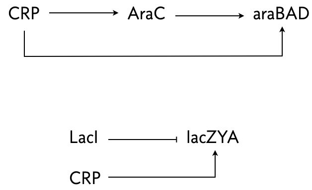
In both system where multiple species regulate one, AND logic is employed.

Mangan an coworkers (J. Molec. Biol., 2003) performed an experiment where they put a fluorescent reporter under control of the products of these two systems, araBAD and lacZYA, respectively. In the lac system, IPTG was also present, so LacI was inhibited. Thus, lacZYA production was directly activated by CRP. Conversely, the arabinose system is a C1-FFL.

They measured the fluorescent intensity in cells that were suddenly exposed to cAMP. The response of these two systems to the sudden jump in cAMP is shown in the left plot below.

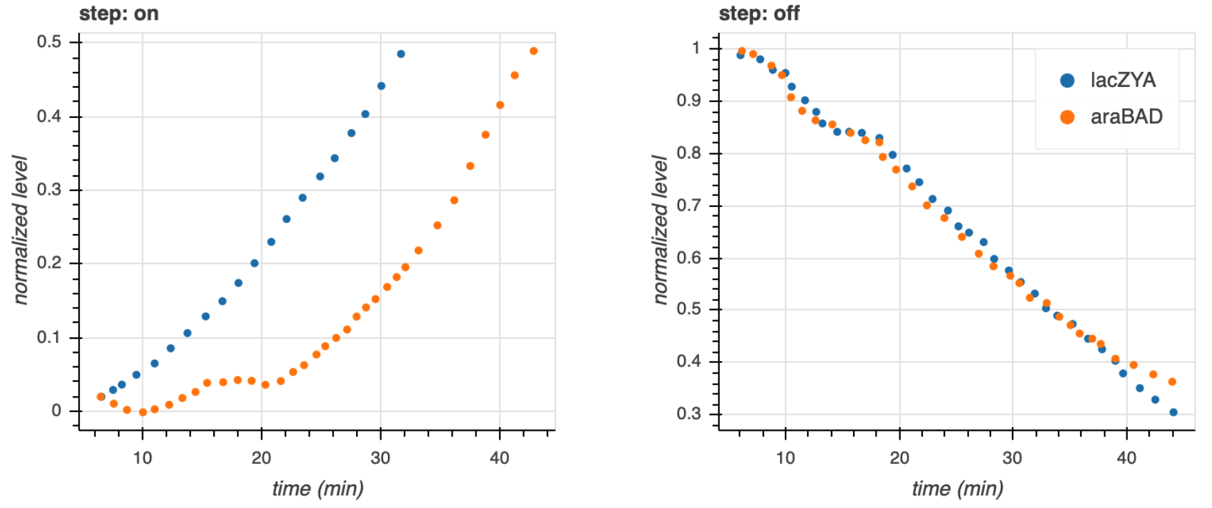
While the lac system response immediately, the arabinose system exhibits a lag before responding. This is indicative of a time delay for a step on in the stimulus for a C1-FFL. Conversely, after these systems come to steady state and are subjected to a sudden decrease in cAMP, both the arabinose and lac systems respond immediately, without delay, which is also expected from a C1-FFL with AND logic.

Kalir and coworkers (Mol. Sys. Biol., 2005) did a similar experiment with another C1-FFL circuit found in E. coli, this time with OR logic. A circuit that regulates flagella formation is a “decorated” C1-FFL, shown below. We say it is decorated because the “Y” gene, in this case FliA, is also autoregulated. Importantly, the regulation of FliL by FliA and FlhDC is governed by OR logic.

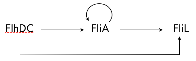
Kalir and coworkers used engineered cells in which the FlhDC gene was under control of a promoter which could be induced with L-arabinose, a chemical inducer. The gene product FliL was altered to be fused to GFP to enable fluorescent monitoring of expression levels. To consider a circuit where FlhDC directly activates FliL, Kalir and coworkers used mutant E. coli cells in which the fliA gene was deleted.

Because of the OR logic, we would expect that a sudden increase in FlhDC would result in both the wild type and mutant cells to respond at the same time, that is with no delay. Fluorescence traces from these experiments are shown in the left plot, below.

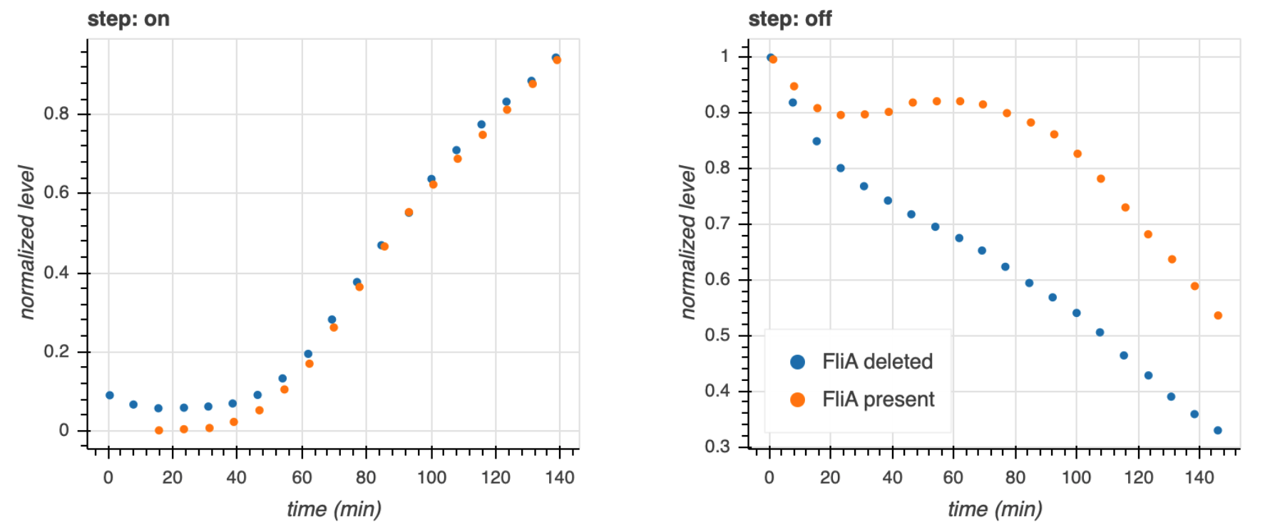
Both strains show a delay, which is due to waiting for FlhDC to be activated, but both come on at the same time. Conversely, after the inducer is removed and FlhDC levels go down, the system with the wild type C1-FFL circuit shows a delay before the FliL levels drop off, while the mutant does not. This demonstrates the sign-sensitivity with OR logic.

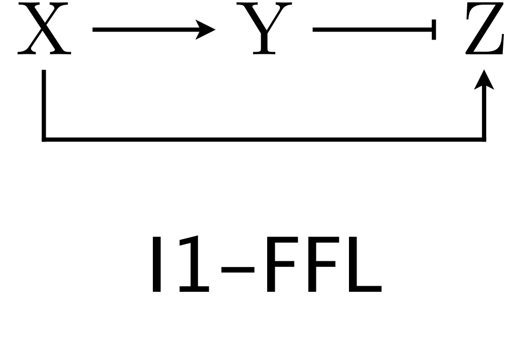
The I1-FFL with AND logic is a pulse generator

We now turn our attention to the other over-represented circuit, the I1-FFL. As a reminder, here is the structure of the circuit.

X activates Y and Z, but Y represses Z. We can use the expressions for production rate under AND and OR logic for one activator/one repressor that we showed above in writing down our dynamical equations. Here, we will consider AND logic. The dimensionless dynamical equations are

\begin{align} \frac{\mathrm{d}y}{\mathrm{d}t} &= \beta\,\frac{(\kappa x)^{n_{xy}}}{1+(\kappa x)^{n_{xy}}} - y,\\[1em] \gamma^{-1}\,\frac{\mathrm{d}z}{\mathrm{d}t} &= \frac{x^{n_{xz}}}{(1 + x^{n_{xz}} + y^{n_{yz}})} - z. \end{align}

For this circuit, we will investigate the response in Z to a sudden, sustained step in stimulus X. We will choose \(\gamma = 10\), which means that the dynamics of Z are faster than Y.

# Parameter values
beta = 5
gamma = 10
kappa = 1
n_xy, n_yz = 3, 3
n_xz = 5
t = np.linspace(0, 10, 200)

# Set up and solve
bokeh.io.show(
    plot_ffl(
        beta,
        gamma,
        kappa,
        n_xy,
        n_xz,
        n_yz,
        ffl="i1",
        logic="and",
        t=t,
        t_step_down=np.inf,
        normalized=False,
    )
)

We see that Z pulses up and then falls down to its steady state value. This is because the presence X leads to production of Z due to its activation. X also leads to the increase in Y, and once enough Y is present, it can start to repress Z. This brings the Z level back down toward a new steady state where the production rate of Z is a balance between activation by X and repression by Y. Thus, the I1-FFL with AND logic is a pulse generator.

The I1-FFL with AND logic gives an accelerated response

Let us compare the response of an I1-FFL being suddenly turned on (by a step in X) to an unregulated circuit that achieves the same steady state. Recall that the dimensionless dynamics for the unregulated circuit follow

\begin{align} z(t) = 1 - \mathrm{e}^{-t}. \end{align}

If we plot the normalized I1-FFL together with the unregulated response, we see that the I1-FFl makes it to the steady state faster, though it overshoots and then relaxes.

p = bokeh.plotting.figure(
    frame_height=200,
    frame_width=550,
    x_axis_label="dimensionless time",
    y_axis_label="dimensionless conc.",
    x_range=[0, 10],
)

# I1-FFL dynamics
yz = solve_ffl(
    beta, gamma, kappa, n_xy, n_xz, n_yz, "i1", "and", t, np.inf, 1
)
p.line(
    t,
    yz[:, 1] / yz[-1, 1],
    line_width=2,
    color=colors[2],
    legend_label="I1-FFL",
)

# Unregulated dynamics
p.line(
    t,
    1 - np.exp(-t),
    line_width=2,
    color=colors[4],
    legend_label="unregulated",
)

bokeh.io.show(p)

So, we have another design principle, The I1-FFL with AND logic has a faster response time than an unregulated circuit.

The accelerated response of the I1-FFL is observed experimentally

Mangan and coworkers (J. Mol. Biol., 2006) investigated an I1-FFL circuit that E. coli uses in its galactose utilization system. The circuit is shown below.

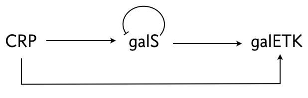
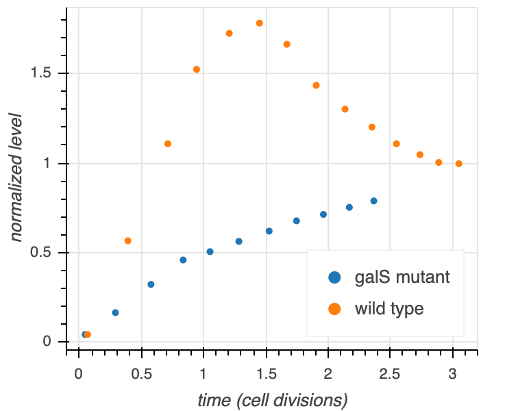
As the “X” gene in this I1-FFL is CRP, the circuit is induced by sudden addition of cAMP, as in the arabidose and lactose circuits above. Mangan and coworkers investigated the response of the wild type circuit, as well as a mutant circuit where galS was deleted. This latter circuit lacks the feed forward loop, and the production of galETK is directly regulated by CRP.

In their experiment, the galE promoter was engineering to express GFP so they could monitor the dynamics of the circuit with fluorescence. The result is shown below. We see that indeed the wild type I1-FFL architecture speeds up the response to the cAMP input, complete with the overshoot we expect from an I1-FFL circuit.

Dashboard

Finally, to enable exploration of FFL’s we construct a dashboard to explore the dynamics. We start by defining our sliders.

param_sliders_kwargs = dict(start=0.1, end=10, step=0.1, value=1)
hill_coeff_kwags = dict(start=0.1, end=10, step=0.1, value=1)

beta_slider = pn.widgets.FloatSlider(name="β", **param_sliders_kwargs)
gamma_slider = pn.widgets.FloatSlider(name="γ", **param_sliders_kwargs)
kappa_slider = pn.widgets.FloatSlider(name="κ", **param_sliders_kwargs)
n_xy_slider = pn.widgets.FloatSlider(name="nxy", **hill_coeff_kwags)
n_xz_slider = pn.widgets.FloatSlider(name="nxz", **hill_coeff_kwags)
n_yz_slider = pn.widgets.FloatSlider(name="nyz", **hill_coeff_kwags)
ffl_selector = pn.widgets.Select(
    name="Circuit",
    options=[
        f"{x}-FFL" for x in ["C1", "C2", "C3", "C4", "I1", "I2", "I3", "I4"]
    ],
    value="C1-FFL",
)
logic_selector = pn.widgets.RadioBoxGroup(
    name="Logic", options=["AND", "OR"], value="AND", inline=True
)
t_step_down_slider = pn.widgets.FloatSlider(
    name="step down time", start=0.1, end=21, step=0.1, value=10
)
x_0_slider = pn.widgets.FloatSlider(
    name="x₀", start=0.1, end=10, step=0.1, value=1
)
normalize_checkbox = pn.widgets.Checkbox(name="Normalize", value=False)

Next, we add the decorator to our plot_ffl() function to enable interactivity. We have to recopy the function to enable addition of the decorator. This is a disadvantage of using our pn.depends() decorator approach to building dashboards; the function definition for making the plot has to be built together with the widgets that control it. You can read about other ways to implement interactions with Panel, along with pros and cons, here. I generally prefer the decorator approach, despite having the redefine functions within the pedagogical context of these notebooks.

@pn.depends(
    beta_slider.param.value,
    gamma_slider.param.value,
    kappa_slider.param.value,
    n_xy_slider.param.value,
    n_xz_slider.param.value,
    n_yz_slider.param.value,
    ffl_selector.param.value,
    logic_selector.param.value,
    t_step_down=t_step_down_slider.param.value,
    x_0=x_0_slider.param.value,
    normalized=normalize_checkbox.param.value,
)
def plot_ffl(
    beta=1,
    gamma=1,
    kappa=1,
    n_xy=1,
    n_xz=1,
    n_yz=1,
    ffl="c1",
    logic="and",
    t=np.linspace(0, 20, 200),
    t_step_down=10,
    x_0=1,
    normalized=False,
):
    yz = solve_ffl(
        beta, gamma, kappa, n_xy, n_xz, n_yz, ffl, logic, t, t_step_down, x_0
    )
    y, z = yz.transpose()

    # Generate x-values
    if t[-1] > t_step_down:
        t_x = np.array(
            [-t_step_down / 10, 0, 0, t_step_down, t_step_down, t[-1]]
        )
        x = np.array([0, 0, x_0, x_0, 0, 0])
    else:
        t_x = np.array([-t[-1] / 10, 0, 0, t[-1]])
        x = np.array([0, 0, x_0, x_0])

    # Add left part of y and z-values
    t = np.concatenate(((t_x[0],), t))
    y = np.concatenate(((0,), y))
    z = np.concatenate(((0,), z))

    # Set up figure
    p = bokeh.plotting.figure(
        frame_height=175,
        frame_width=550,
        x_axis_label="dimensionless time",
        y_axis_label=f"{'norm. ' if normalized else ''}dimensionless conc.",
        x_range=[t.min(), t.max()],
    )

    if normalized:
        p.line(
            t_x, x / x.max(), line_width=2, color=colors[0], legend_label="x"
        )
        p.line(
            t, y / y.max(), line_width=2, color=colors[1], legend_label="y",
        )
        p.line(
            t, z / z.max(), line_width=2, color=colors[2], legend_label="z",
        )
    else:
        p.line(t_x, x, line_width=2, color=colors[0], legend_label="x")
        p.line(t, y, line_width=2, color=colors[1], legend_label="y")
        p.line(t, z, line_width=2, color=colors[2], legend_label="z")

    p.legend.click_policy = "hide"

    return p

Finally, we build the dashboard by laying out the plot and widgets.

sliders = pn.Row(
    pn.Spacer(width=30),
    pn.Column(beta_slider, gamma_slider, kappa_slider, width=150),
    pn.Spacer(width=10),
    pn.Column(n_xy_slider, n_xz_slider, n_yz_slider, width=150),
    pn.Spacer(width=10),
    pn.Column(t_step_down_slider, x_0_slider, width=150),
)

selectors = pn.Column(
    ffl_selector, logic_selector, normalize_checkbox, width=150
)

# Final layout
pn.Column(
    plot_ffl,
    pn.Spacer(width=10),
    pn.Row(sliders, pn.Spacer(width=10), selectors),
)

Data type cannot be displayed:

By playing with the widgets, you can see what parameter ranges give the behaviors we outlined in our preceding discussion on genetic circuits.

Computing environment

%load_ext watermark
%watermark -v -p numpy,scipy,panel,bokeh,jupyterlab

CPython 3.7.7
IPython 7.13.0

numpy 1.18.1
scipy 1.4.1
panel 0.9.5
bokeh 2.0.2
jupyterlab 1.2.6