20. Turing patterns
Design principle
Local activation and long range inhibition can give stable, spatially heterogeneous patterning of morphogens.
Concepts
Reaction-diffusion equations
Techniques
Numerical solution of PDEs by the method of lines
Linear stability analysis of PDEs
[1]:
import numpy as np
import pandas as pd
import numba
import scipy.integrate
import biocircuits
import bokeh.io
import bokeh.plotting
import panel as pn
pn.extension()
bokeh.io.output_notebook()
Note: To run this notebook, you will need to update biocircuits.
pip install --upgrade biocircuits
At the end of the notebook, we solve a two-dimensional reaction-diffusion system. If you wish to do that calculation, you also need to install rdsolver.
pip install rdsolver
In recent lectures, we have been talking about signaling between cells, whether via cytokines regulating homeostasis, via Delta-Notch signaling, or via BMP signaling. The latter two signaling pathways are important in development of an organism, as we saw in lecture. They lead to spatial patterning of cells of different types.
As we saw in the discussion of BMP, the expression of other genes in the cells of interest depend on the concentration of the ligands and receptors involved in signaling. It seems that in many contexts, biochemical cues that influence cell fate do so in a concentration-dependent manner; higher concentrations result in stronger signals than lower concentrations. Such chemical species, which determine cell fate in a developmental context in a concentration-dependent way, are called morphogens.
For this lecture, we will discuss reaction-diffusion mechanisms for generating spatial distributions of morphogens. This is important both practically and historically.
Turing’s thoughts on reaction-diffusion mechanisms for morphogenesis
In his landmark paper (Turing, 1952), Alan Turing laid out a prescription for morphogenesis. He described what should be considered when studying the “changes of state” of a developing organism. Turing said,
In determining the changes of state one should take into account:
the changes of position and velocity as given by Newton’s laws of motion;
the stresses as given by the elasticities and motions, also taking into account the osmotic pressures as given from the chemical data;
the chemical reactions;
the diffusion of the chemical substances (the region in which this diffusion is possible is given from the mechanical data).
This makes perfect sense; it we are shaping an organism, we have to think about what changes the shape and also how the little molecules that govern the shape move about and react. That said, a few lines later in the paper, Turing wrote, “The interdependence of the chemical and mechanical data adds enormously to the difficulty, and attention will therefore be confined, so far as is possible, to cases where these can be separated.”
Turing went on to consider only the chemical reactions coupled with diffusion. His claim, which we will explore mathematically in this lecture, was that when diffusion was considered, spatial patterns in chemical species could form. Stop and think about that for a moment. Diffusion, a dissipative process, can help give spatial patterns in chemical systems that otherwise have no spatial information. In all of your life experience, I bet diffusion has served to flatten out patterns, like when you put food coloring in a glass of water. Let’s explore Turing’s counterintuitive proposal.
We will specifically explore a type of patterning that now bears the name “Turing patterns.” A Turing pattern is formed spontaneously due to diffusion from a system of two chemical species that have a stable fixed point in the absence of diffusion.
Reaction-diffusion equations for two components
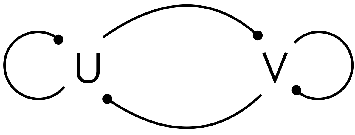
Consider two chemical components, U and V, that can react with each other. The dynamical equations we have considered thus far are of the form
\begin{align} \frac{\mathrm{d}u}{\mathrm{d}t} &= f(u, v)\\[1em] \frac{\mathrm{d}v}{\mathrm{d}t} &= g(u, v). \end{align}
If the species can undergo diffusion, we need to include diffusive terms. We use Fick’s second law, which says that the rate of change of concentration of a diffusing species is
\begin{align} \frac{\partial c}{\partial t} = D\nabla^2 c, \end{align}
to update our dynamical equations.
\begin{align} \frac{\partial u}{\partial t} &= D_u\nabla^2 u + f(u, v)\\[1em] \frac{\partial v}{\partial t} &= D_v\nabla^2 v + g(u, v). \end{align}
Our goal is to determine what type of regulation we need in the chemical circuit (i.e., to decide what type of arrowheads, activating or repressing, to use in the figure below, and what values of \(D_u\) and \(D_v\) are necessary to give spontaneous patterning of U and V).
Linear stability analysis of a PDE
Earlier in the class, we learned how to do linear stability analysis of a fixed point of a system of ordinary differential equations. For this system, we also have spatial derivatives, so we need to perform linear stability analysis on a system of partial differential equations. Specifically, we will consider a chemical reaction system that has a stable fixed point in the absence of diffusion. The idea is that the chemical reaction system itself will not be oscillatory and run away to some other state. We will test to see if the inclusion of spatial information, by explicitly considering diffusion, can make the entire system unstable, thereby giving rise to patterns.
Let us assume that \((u_0, v_0)\) is a stable fixed point of the dynamical system in the absence of diffusion. That is, \(f(u_0, v_0) = g(u_0, v_0) = 0\). Therefore, we can construct a homogeneous steady state where \(a(\mathbf{x}) = u_0\) and \(b(\mathbf{x}) = v_0\), where \(\mathbf{x}\) denotes spatial variables. This is to say that the concentrations of species \(u\) and \(v\) are everywhere equal to their value at the stable fixed point. This is the unpatterned state, which is stable in the absence of diffusion.
The question now is is the homogeneous steady state stable in the presence of diffusion? To answer this question, we will perform a linear stability analysis. We linearize \(f(u, v)\) and \(g(u, v)\) about \((u_0, v_0)\).
\begin{align} f(u, v) \approx f(u_0, v_0) + f_u \delta u + f_v\delta v,\\[1em] g(u, v) \approx g(u_0, v_0) + g_u\delta u + g_v\delta v, \end{align}
where
\begin{align} f_u &= \left.\frac{\partial f}{\partial u}\right|_{(u_0, v_0)}, \;\; f_v = \left.\frac{\partial f}{\partial v}\right|_{(u_0, v_0)}, \\[1em] g_u &= \left.\frac{\partial g}{\partial u}\right|_{(u_0, v_0)}, \;\; g_v = \left.\frac{\partial g}{\partial v}\right|_{(u_0, v_0)}, \end{align}
and \(\delta u = u - u_0\) and \(\delta v = v - v_0\) represent the perturbation from the homogeneous steady state. Note that \(\delta u\) and \(\delta v\) are functions of position \(\mathbf{x}\) and time \(t\). Thus, our linearized system is
\begin{align} \frac{\partial \delta u}{\partial t} &= D_u\nabla^2 \delta u + f_u\delta u + f_v\delta v, \\[1em] \frac{\partial \delta v}{\partial t} &= D_v\nabla^2 \delta v + g_u\delta u + g_v\delta v. \end{align}
Note that the terms \(f_u\) and \(g_v\) describe the nature of the autoregulation of the genetic circuit
Taking the Fourier transform of the equations gives
\begin{align} \frac{\partial \widehat{\delta u}}{\partial t} &= -k^2D_u \widehat{\delta u} + f_u\widehat{\delta u} + f_v\widehat{\delta v} \\ \frac{\partial \widehat{\delta v}}{\partial t} &= -k^2D_v \widehat{\delta v} + g_u\widehat{\delta u} + g_v\widehat{\delta v}, \end{align}
where \(\mathbf{k}\) is the vector of wave numbers (e.g., \(\mathbf{k} = (k_x, k_y)\) for a two-dimensional system) and \(k^2 \equiv \mathbf{k}\cdot \mathbf{k}\). This is now a system of linear ordinary differential equations in \(\widehat{\delta u}\) and \(\widehat{\delta v}\), which we can approach in our usual way of doing linear stability analysis.
To avoid the cumbersome hats on the Fourier-transformed variables, we note that solving the linear system above is the same as searching for harmonic solutions to equations to the linearized PDEs describing the perturbations \(\delta u\) and \(\delta v\) of the form
\begin{align} \delta u &= \delta u_0 \, \mathrm{e}^{-i\mathbf{k}\cdot\mathbf{x} + \lambda t},\\[1em] \delta v &= \delta v_0 \, \mathrm{e}^{-i\mathbf{k}\cdot\mathbf{x} + \lambda t}. \end{align}
We can then write the resulting system of linear ODEs as
\begin{align} \lambda \begin{pmatrix} \delta u\\ \delta v \end{pmatrix} = \mathsf{A}\,\begin{pmatrix} \delta u\\ \delta v \end{pmatrix}, \end{align}
where the linear stability matrix is given by
:nbsphinx-math:`begin{align} mathsf{A} = begin{pmatrix} -k^2D_u + f_u & f_v \
g_u & -k^2D_v + g_v
end{pmatrix}. end{align}`
As before, our goal is to compute the eigenvalues \(\lambda\) of this matrix. For a 2$:nbsphinx-math:`times`$2 matrix, the eigenvalues are
\begin{align} \lambda = \frac{1}{2}\left(\mathrm{tr}(\mathsf{A}) \pm \sqrt{\mathrm{tr}^2(\mathsf{A}) - 4\mathrm{det}(\mathsf{A})}\right), \end{align}
where \(\mathrm{tr}(\mathsf{A})\) is the trace of \(\mathsf{A}\) and \(\mathrm{det}(\mathsf{A})\) is its determinant.
In the absence of diffusion, \(\mathrm{tr}(\mathsf{A}) = f_u + g_v\). Because we have specified that in the absence of diffusion, the chemical reaction system has a stable fixed point, at least one of \(f_u\) or \(g_v\) must be negative. Interestingly, the trace of the linear stability matrix with diffusion included is maximal for the zeroth mode (\(k = 0\)), which means that an instability arising from the trace becoming positive has the zeroth mode as its fastest growing. If the determinant is positive at the onset of the instability (when the trace crosses zero), the eigenvalues are imaginary, which means that the zeroth mode is oscillatory. This is called a Hopf bifurcation.
We will stipulate that \(g_v < 0\), leaving for now the possibility that \(f_u\) may be negative as well. In the presence of diffusion, the trace is
\begin{align} \mathrm{tr}(\mathsf{A}) = f_u + g_v - \left(D_u + D_v\right)k^2. \end{align}
Since the second term is always negative, and we have decreed that \(f_u + g_v < 0\) by virtue of the chemical reaction system being stable in the absence of diffusion, the trace is always negative. As such, we can only get an eigenvalue with a positive real part (an instability) if the determinant is negative.
The determinant of the linear stability matrix is
\begin{align} \mathrm{det}(\mathsf{A}) = D_uD_v\,k^4 - (D_v\,f_u + D_u\, g_v)k^2 + f_u \,g_v - f_v\, g_u. \end{align}
This is quadratic in \(k^2\), and since \(D_u D_v > 0\), this is a convex parabola. Therefore, we can calculate the wave number where the parabola is a minimum.
\begin{align} \frac{\partial}{\partial k^2} \,\mathrm{det}(\mathsf{A}) = 2D_u D_v \,k^2 - D_v f_u - D_u g_v = 0. \end{align}
Thus, we have
\begin{align} k^2_\mathrm{min} = \frac{D_u\, g_v + D_v \,f_u}{2D_u D_v}. \end{align}
Inserting this expression into the expression for the determinant gives the minimal value of the determinant.
\begin{align} \mathrm{det}(\mathsf{A}(k_\mathrm{min})) = f_u g_v - f_v g_u - \frac{(D_u\,g_v + D_v\,f_u)^2}{4D_u D_v}. \end{align}
Therefore, the determinant is negative when
\begin{align} D_u \,g_v + D_v\,f_u > 2\sqrt{D_uD_v(f_u g_v - f_v g_u)}. \end{align}
Because the above inequality must hold to get a negative determinant and therefore an instability, so too must the less restrictive inequality
\begin{align} D_u\,g_v + D_v\,f_u > 0 \end{align}
hold. Since we already showed that at least one of \(f_u\) or \(g_v\) must be negative, we must have exactly one be negative. We will take \(f_u > 0\), as we already decreed that \(g_v < 0\).
Because we have decreed that the chemical system in the absence of diffusion is stable, the determinant of the linear stability matrix of the diffusion-less system, \(f_u g_v - f_v g_u\), must be positive. Because \(f_u g_v < 0\), we must also have \(f_v g_u < 0\). This means that the activator must be involved in a negative feedback loop. That is, if U activates V (\(f_v > 0\)), then V must repress U (\(g_u < 0\)), and vice versa.
Note that having \(g_v < 0\) does not necessarily mean that we have autoinhibition, since we could also have \(g_v < 0\) by degradation or dilution. However, the signs of \(f_u\) and \(g_v\) indicate that U is autoactivating and is in a negative feedback loop with V.
In summary, we have five inequalities,
\begin{align} &f_u > 0, \\[1em] &g_v < 0, \\[1em] &f_u + g_v < 0,\\[1em] &f_u g_v - f_v g_u > 0 \\[1em] &D_v\,f_u + D_u\,g_v > 0. \end{align}
A requirement for all of these inequalities can only hold is that \(D_v > D_u\). Thus, we have arrived at our conditions for formation of Turing patterns.
We need an autocatalytic species (an “activator”).
The activator must form a negative feedback loop with the other species, the “inhibitor.”
The inhibitor must diffuse more rapidly than the activator.
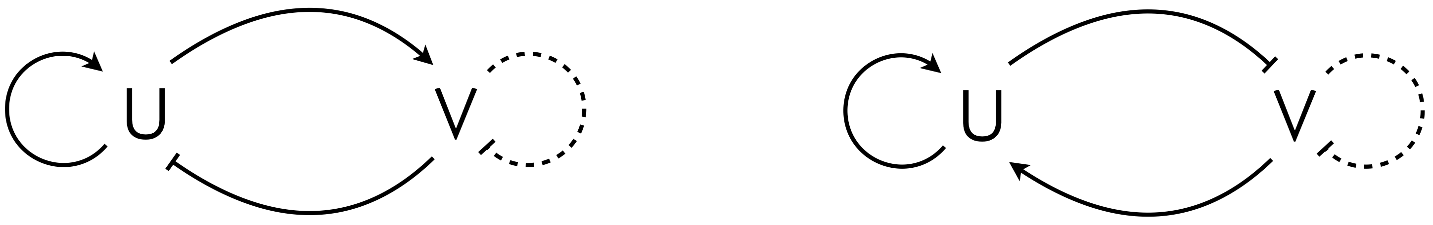
The intuition here is that the activator starts producing more of itself locally. The local peak starts to spread, but the inhibitor diffuses more quickly so that it pins the peak of activator in so that it cannot spread. This gives a set wavelength of the pattern of peaks. The circuits below can lead to Turing patterns. The dashed line indicates that autorepression is not necessary, only that \(g_v < 0\).
Wavelength of a Turing pattern
The wavelength of a Turing pattern is set, at least as the instability begins to grow, by the fastest growing mode, \(k\). That is, for the value of \(k\) for which the eigenvalue \(\lambda\) is largest. We have already shown that \(k_\mathrm{min}\), the \(k\) for which the determinant of the linear stability matrix is minimal, is the \(k\) corresponding to the fastest growing mode.
We can derive a dispersion relation, which relates the eigenvalues of the linear stability matrix \(\mathsf{A}\) to the wave number \(k\). Specifically, is \(\lambda_\mathrm{max}\) is the eigenvalue with the largest real part, the dispersion relation is the function \(\mathrm{Re}[\lambda_\mathrm{max}(k)]\). The dispersion relation describes what modes contribute to the instability; these set the wavelength of the emergent pattern. This is perhaps best understood by example, which we consider below with the activator substrate depletion model.
Turing patterns do not scale
Turing patterns do not scale with the size of the organism because the wavelength of the pattern, given by the fastest growing mode, \(k_\mathrm{min}\), is independent of system size. So, if a system is twice as large, it would have twice as many peaks and valleys in the pattern. In the next lesson, we will address this problem of scaling and talk about reaction-diffusion systems that can give patterns that scale with organism size.
Example: The Activator-Substrate Depletion Model
As an example of a system that undergoes a Turing pattern, let us consider now the activator-substrate depletion model, or ASDM. This is a simple model in which there are two species, the activator and substrate. The activator is autocatalytic, but consumes substrate in the process. It also has our standard degradation. The substrate is constitutively produced, and for the sake of simplicity, we assume it is very stable such that its degradation is all by consumption by the activator. This corresponds to the right circuit in our figure of circuits that can give Turing patterns, above. The dynamical equations are
\begin{align} \frac{\partial a}{\partial t} &= D_a\,\nabla^2 a + \rho a^2s - \gamma a,\\[1em] \frac{\partial s}{\partial t} &= D_s\,\nabla^2 s + \beta - \rho a^2s. \end{align}
We nondimensionalize by choosing \(t \leftarrow t\gamma\), \((x,y,z) \leftarrow \sqrt{D_s/\gamma}(x, y, z)\), \(a \leftarrow \gamma a/\beta\), \(s \leftarrow \beta\rho s/\gamma^2\), \(d = D_a/D_s\) and \(\mu = \beta^2\rho/\gamma^3\). Then, the dimensionless equations are
\begin{align} \frac{\partial a}{\partial t} &= d \nabla^2 a + a^2s - a,\\[1em] \frac{\partial s}{\partial t} &= \nabla^2 s + \mu(1-a^2s). \end{align}
This system has a unique homogeneous steady state of \(a_0 = s_0 = 1\).
The two dimensionless parameters have physical meaning. The parameter \(d\) is the ratio of the diffusion coefficient of the activator to that of the substrate. Small \(d\) means that the substrate diffuses much more rapidly than the activator. The parameter \(\mu\) describes the relative rates of chemical reactions for substrate compared to activator.
In the language of our general Turing system, here we have \(f_a = f_s = 1\), \(g_a = -2\mu\), and \(g_s = -\mu\), so we have a linear stability matrix
\begin{align} \mathsf{A} = \begin{pmatrix} 1-dk^2 & 1 \\ -2\mu & -\mu-k^2 \end{pmatrix}. \end{align}
Dispersion relation
With the linear stability matrix in hand, we can compute and plot the dispersion relation. We will allow for various values of the two parameters \(d\) and \(\mu\). First, we write a function to compute the dispersion relation. It is a function of the wave number \(k\).
[2]:
def dispersion_relation(k_vals, d, mu):
lam = np.empty_like(k_vals)
for i, k in enumerate(k_vals):
A = np.array([[1-d*k**2, 1],
[-2*mu, -mu - k**2]])
lam[i] = np.linalg.eigvals(A).real.max()
return lam
Next, we build an interactive graphic to explore the dispersion relation as we adjust the parameter values \(d\) and \(\mu\).
[3]:
d_slider = pn.widgets.FloatSlider(
name="d", start=0.01, end=1, value=0.05, step=0.01, width=150
)
mu_slider = pn.widgets.FloatSlider(
name="μ", start=0.01, end=2, value=1.5, step=0.005, width=150
)
@pn.depends(d_slider.param.value, mu_slider.param.value)
def plot_dispersion_relation(d, mu):
k = np.linspace(0, 10, 200)
lam_max_real_part = dispersion_relation(k, d, mu)
p = bokeh.plotting.figure(
frame_width=350,
frame_height=200,
x_axis_label="k",
y_axis_label="Re[λ-max]",
x_range=[0, 10],
)
p.line(k, lam_max_real_part, color="black", line_width=2)
return p
pn.Column(
pn.Row(d_slider, mu_slider), pn.Spacer(height=20), plot_dispersion_relation
)
Data type cannot be displayed:
[3]:
By playing with the sliders, we can see that the maximal real part of the eigenvalues is always below zero for large \(d\). For small \(d\), and for \(\mu > 1\), we can get a positive real part of an eigenvalue, with the maximum occurring at \(k = 0\). This implies that the zero mode, or uniform concentration, grows fastest. However, for small \(d\) with \(\mu > 1\), we get a fastest growing mode for finite positive \(k\). In this regimes, we can form patterns.
Linear stability diagram
We have just explored the parameter values that give patterns with interactive plots of the dispersion relation. We can take a similar approach to construct a linear stability diagram. There are two parameters, \(\mu\) and \(d\), and we can imagine a map of the \(d\)-\(\mu\) plane identifying which regions of parameter space that have different linear stability properties. We have five possibilities in this system. Denoting by \(k_\mathrm{max}\) a wavenumber for which the largest real part of the eigenvalues if (locally) maximal, we have the following.
Eigenvalues |
Description |
color |
|---|---|---|
Negative real parts |
Homogeneous steady state stable |
green |
Real, positive, \(k_\mathrm{max}>0\) |
Pattern forming |
purple |
Real, positive, \(k_\mathrm{max} = 0\) |
Homogeneous conc. grows without bound |
blue |
Real, positive, \(k_\mathrm{max} = 0\) and \(k_\mathrm{max} > 0\) |
Possible patterns, depending on initial condition |
yellow |
Imaginary, \(k_\mathrm{max} > 0\) |
Oscillating homogeneous patterns |
orange |
In some cases, we can conveniently compute the boundaries between the different regions of parameter spaces, but it is often easier to take a “brute force” approach, wherein we compute the eigenvalues for each set of parameter values for a range of \(k\)-values, and then display the results as an image colored according to which class of eigenvalues we get. This is implemented below.
[4]:
# Values for the plot
mu_vals = np.linspace(0.001, 2, 400)
d_vals = np.linspace(0.001, 1, 400)
@numba.njit
def region(d, mu):
"""Returns which region the eigenvalue lives in."""
osc = False
unstable = False
turing = False
if 3 - 2 * np.sqrt(2) < mu < 1:
osc = True
k2 = np.linspace(0, 10, 200)
det = (1 - d * k2) * (-mu - k2) + 2 * mu
tr = 1 - (1 + d) * k2 - mu
real_lam = np.empty_like(k2)
for i, (t, d) in enumerate(zip(tr, det)):
discriminant = t ** 2 - 4 * d
if discriminant < 0:
real_lam[i] = t / 2
else:
real_lam[i] = (t + np.sqrt(discriminant)) / 2
if (real_lam > 0).any():
unstable = True
if np.argmax(real_lam) > 0:
turing = True
if osc:
if turing:
return 3
return 2
if unstable:
if turing:
return 1
return 4
return 0
# Compute linear stability diagram
d, mu = np.meshgrid(d_vals, mu_vals)
im = np.empty_like(d)
for i in range(len(mu_vals)):
for j in range(len(d_vals)):
im[i, j] = region(d_vals[j], mu_vals[i])
# Set up the coloring
color_mapper = bokeh.models.LinearColorMapper(
["#7fc97f", "#beaed4", "#fdc086", "#ffff99", "#386cb0"]
)
# Make plot and display
p = biocircuits.imshow(
im,
color_mapper=color_mapper,
x_range=[d.min(), d.max()],
y_range=[mu.min(), mu.max()],
frame_height=300,
x_axis_label="d",
y_axis_label="µ",
flip=False,
display_clicks=True,
)
bokeh.io.show(p)
The “sweet spot” for Turing patterns is in the upper left, small \(d\) (substrate diffuses much more rapidly than activator) and large \(\mu\) (fast chemical reactions).
Note that the above diagram only describes the dynamics in the linear regime. For example, in the orange region, the instability may be oscillatory, but the system may not have a stable limit cycle, meaning that it will not oscillate continuously.
Numerical solution of R-D PDEs
We now turn to numerical solutions of the partial differential equations describing the reaction-diffusion system.
Tissue size
We will solve the PDEs on the domain \(0 \le x \le L\), where \(L\) is the total length of the growing tissue. We did not consider a finite domain size when we were doing the linear stability analysis. If all wave numbers \(k\) for which an eigenvalue has positive real part are larger than the domain size \(L\), the domain cannot accommodate the nascent pattern. In this case the homogeneous steady state remains stable.
This is another mechanism by which a reaction-diffusion system can give patterns. As a tissue grows, when it passes a length that can accommodate the pattern, the pattern can spontaneously form.
Boundary conditions
For any set of PDEs, we need to also specify boundary and initial conditions. We can choose periodic boundary conditions, \(c(0,t) = c(L,t)\), where \(c\) is the concentration of a morphogen. This is appropriate, for example, in examining patterning around a cylinder, which was the case in the Turing paper in looking at the pattering of developing whorl around a stem.
We may also want to consider no-flux boundary conditions, in which the flux of morphogen at the boundaries is zero. This is the case for a tissue of finite size; the morphogen cannot diffuse off of the end of the tissue. The diffusive flux, as given by Fick’s Law is
\begin{align} j(x) = -D\,\frac{\partial c}{\partial x}. \end{align}
So, a no-flux condition means that we set the first derivative of the concentration profile to zero at the boundaries. In what follows, we will use no-flux conditions.
Mechanics of the numerical solution
To investigate the dynamics of spontaneously forming patterns, we need to solve the governing PDEs numerically. We will use a technique known as the method of lines to do so. The idea is that we discretize the spatial coordinate \(x\) in evenly spaced points with spacing \(\Delta x\) between each point. To compute the second derivatives that come about in the diffusion terms, we use central differencing. In the central differencing scheme, we approximate the second derivative of a concentration evaluated at point \(x_i\) (which is one of our discrete grid points) as
\begin{align} \left.\frac{\partial^2 c}{\partial x^2}\right|_{x=x_i} \approx \frac{c(x_{i+1}) + c(x_{i-1}) - 2c(x_i)}{\Delta x^2}. \end{align}
By discretizing the spatial variable, we now have a system of ordinary differential equations. In this case, where we have two species, we have two times the number of grid points ordinary differential equations. We can then use scipy.integrate.odeint() to solve this system.
This is implemented in the functions below, which also allow for nonconstant diffusion coefficients.
[5]:
def dc_dt(
c,
t,
x,
derivs_0,
derivs_L,
diff_coeff_fun,
diff_coeff_params,
rxn_fun,
rxn_params,
n_species,
h,
):
"""
Time derivative of concentrations in an R-D system
for constant flux BCs.
Parameters
----------
c : ndarray, shape (n_species * n_gridpoints)
The concentration of the chemical species interleaved in a
a NumPy array. The interleaving allows us to take advantage
of the banded structure of the Jacobian when using the
Hindmarsh algorithm for integrating in time.
t : float
Time.
derivs_0 : ndarray, shape (n_species)
derivs_0[i] is the value of the diffusive flux,
D dc_i/dx, at x = 0, the leftmost boundary of the domain of x.
derivs_L : ndarray, shape (n_species)
derivs_0[i] is the value of the diffusive flux,
D dc_i/dx, at x = L, the rightmost boundary of the domain of x.
diff_coeff_fun : function
Function of the form diff_coeff_fun(c_tuple, t, x, *diff_coeff_params).
Returns an tuple where entry i is a NumPy array containing
the diffusion coefficient of species i at the grid points.
c_tuple[i] is a NumPy array containing the concentrations of
species i at the grid poitns.
diff_coeff_params : arbitrary
Tuple of parameters to be passed into diff_coeff_fun.
rxn_fun : function
Function of the form rxn_fun(c_tuple, t, *rxn_params).
Returns an tuple where entry i is a NumPy array containing
the net rate of production of species i by chemical reaction
at the grid points. c_tuple[i] is a NumPy array containing
the concentrations of species i at the grid poitns.
rxn_params : arbitrary
Tuple of parameters to be passed into rxn_fun.
n_species : int
Number of chemical species.
h : float
Grid spacing (assumed to be constant)
Returns
-------
dc_dt : ndarray, shape (n_species * n_gridpoints)
The time derivatives of the concentrations of the chemical
species at the grid points interleaved in a NumPy array.
"""
# Tuple of concentrations
c_tuple = tuple([c[i::n_species] for i in range(n_species)])
# Compute diffusion coefficients
D_tuple = diff_coeff_fun(c_tuple, t, x, *diff_coeff_params)
# Compute reaction terms
rxn_tuple = rxn_fun(c_tuple, t, *rxn_params)
# Return array
conc_deriv = np.empty_like(c)
# Convenient array for storing concentrations
da_dt = np.empty(len(c_tuple[0]))
# Useful to have square of grid spacing around
h2 = h ** 2
# Compute diffusion terms (central differencing w/ Neumann BCs)
for i in range(n_species):
# View of concentrations and diffusion coeff. for convenience
a = np.copy(c_tuple[i])
D = np.copy(D_tuple[i])
# Time derivative at left boundary
da_dt[0] = D[0] / h2 * 2 * (a[1] - a[0] - h * derivs_0[i])
# First derivatives of D and a
dD_dx = (D[2:] - D[:-2]) / (2 * h)
da_dx = (a[2:] - a[:-2]) / (2 * h)
# Time derivative for middle grid points
da_dt[1:-1] = D[1:-1] * np.diff(a, 2) / h2 + dD_dx * da_dx
# Time derivative at left boundary
da_dt[-1] = D[-1] / h2 * 2 * (a[-2] - a[-1] + h * derivs_L[i])
# Store in output array with reaction terms
conc_deriv[i::n_species] = da_dt + rxn_tuple[i]
return conc_deriv
def rd_solve(
c_0_tuple,
t,
L=1,
derivs_0=0,
derivs_L=0,
diff_coeff_fun=None,
diff_coeff_params=(),
rxn_fun=None,
rxn_params=(),
rtol=1.49012e-8,
atol=1.49012e-8,
):
"""
Parameters
----------
c_0_tuple : tuple
c_0_tuple[i] is a NumPy array of length n_gridpoints with the
initial concentrations of chemical species i at the grid points.
t : ndarray
An array of time points for which the solution is desired.
L : float
Total length of the x-domain.
derivs_0 : ndarray, shape (n_species)
derivs_0[i] is the value of dc_i/dx at x = 0.
derivs_L : ndarray, shape (n_species)
derivs_L[i] is the value of dc_i/dx at x = L, the rightmost
boundary of the domain of x.
diff_coeff_fun : function
Function of the form diff_coeff_fun(c_tuple, x, t, *diff_coeff_params).
Returns an tuple where entry i is a NumPy array containing
the diffusion coefficient of species i at the grid points.
c_tuple[i] is a NumPy array containing the concentrations of
species i at the grid poitns.
diff_coeff_params : arbitrary
Tuple of parameters to be passed into diff_coeff_fun.
rxn_fun : function
Function of the form rxn_fun(c_tuple, t, *rxn_params).
Returns an tuple where entry i is a NumPy array containing
the net rate of production of species i by chemical reaction
at the grid points. c_tuple[i] is a NumPy array containing
the concentrations of species i at the grid poitns.
rxn_params : arbitrary
Tuple of parameters to be passed into rxn_fun.
rtol : float
Relative tolerance for solver. Default os odeint's default.
atol : float
Absolute tolerance for solver. Default os odeint's default.
Returns
-------
c_tuple : tuple
c_tuple[i] is a NumPy array of shape (len(t), n_gridpoints)
with the initial concentrations of chemical species i at
the grid points over time.
Notes
-----
.. When intergrating for long times near a steady state, you
may need to lower the absolute tolerance (atol) because the
solution does not change much over time and it may be difficult
for the solver to maintain tight tolerances.
"""
# Number of grid points
n_gridpoints = len(c_0_tuple[0])
# Number of chemical species
n_species = len(c_0_tuple)
# Grid spacing
h = L / (n_gridpoints - 1)
# Grid points
x = np.linspace(0, L, n_gridpoints)
# Set up boundary conditions
if np.isscalar(derivs_0):
derivs_0 = np.array(n_species * [derivs_0])
if np.isscalar(derivs_L):
derivs_L = np.array(n_species * [derivs_L])
# Set up parameters to be passed in to dc_dt
params = (
x,
derivs_0,
derivs_L,
diff_coeff_fun,
diff_coeff_params,
rxn_fun,
rxn_params,
n_species,
h,
)
# Set up initial condition
c0 = np.empty(n_species * n_gridpoints)
for i in range(n_species):
c0[i::n_species] = c_0_tuple[i]
# Solve using odeint, taking advantage of banded structure
c = scipy.integrate.odeint(
dc_dt,
c0,
t,
args=params,
ml=n_species,
mu=n_species,
rtol=rtol,
atol=atol,
)
return tuple([c[:, i::n_species] for i in range(n_species)])
The rd_solve() function is included in the biocircuits package.
Let us proceed to set up and solve for the ASDM model. We will specify an initial condition that is a tiny perturbation from the homogeneous steady state of \(a = s = 1\).
[6]:
def constant_diff_coeffs(c_tuple, t, x, diff_coeffs):
n = len(c_tuple[0])
return tuple([diff_coeffs[i] * np.ones(n) for i in range(len(c_tuple))])
def asdm_rxn(as_tuple, t, mu):
"""
Reaction expression for activator-substrate depletion model.
Returns the rate of production of activator and substrate, respectively.
r_a = a**2 * s - a
r_s = mu * (1 - a**2 * s)
"""
# Unpack concentrations
a, s = as_tuple
# Compute and return reaction rates
a2s = a ** 2 * s
return (a2s - a, mu * (1.0 - a2s))
# Set up steady state (using 500 grid points)
a_0 = np.ones(500)
s_0 = np.ones(500)
# Make a small perturbation to a_0
a_0 += 0.001 * np.random.rand(len(a_0))
# Time points
t = np.linspace(0.0, 1000.0, 100)
# Physical length of system
L = 20.0
# x-coordinates for plotting
x = np.linspace(0, L, len(a_0))
# Diffusion coefficients
diff_coeffs = (0.05, 1.0)
# Reaction parameter (must be a tuple of params, even though only 1 for ASDM)
rxn_params = (1.5,)
# Solve
conc = rd_solve(
(a_0, s_0),
t,
L=L,
derivs_0=0,
derivs_L=0,
diff_coeff_fun=constant_diff_coeffs,
diff_coeff_params=(diff_coeffs,),
rxn_fun=asdm_rxn,
rxn_params=rxn_params,
)
We can now make an interactive plot with a time slider to investigate the dynamics.
[7]:
t_slider = pn.widgets.FloatSlider(
name="t", start=t[0], end=t[-1], value=t[-1], step=t[1] - t[0]
)
@pn.depends(t_slider)
def plot_turing(t_point):
i = np.searchsorted(t, t_point)
p = bokeh.plotting.figure(
frame_width=400,
frame_height=200,
x_axis_label="x",
y_axis_label="a, s",
x_range=[0, L],
y_range=[0, np.concatenate(conc).max()*1.02],
)
p.line(x, conc[0][i, :], legend_label="activator", line_width=2)
p.line(
x,
conc[1][i, :],
color="tomato",
legend_label="substrate",
line_width=2,
)
return p
pn.Column(t_slider, plot_turing)
Data type cannot be displayed:
[7]:
It is useful to quickly make plots like this, so the xyt_plot() function is included in the biocircuits package. It generates a plot of curves that can vary over time and provides a slider to adjust the time variable.
[8]:
bokeh.io.show(
biocircuits.xyt_plot(
x,
conc,
t,
legend_names=["activator", "substrate"],
palette=["#1f77b4", "tomato"],
)
)
Two-dimensional solutions
Using more sophisticated numerical integration techniques, we can solve the ADSM in two dimensions. This is implemented in the rdsolver package, which solves two-dimensional reaction-diffusion problems using spectral methods with implicit-explicit (IMEX) time stepping. For fun, we demonstrate it here.
[9]:
import rdsolver
notebook_url = 'localhost:8888'
# Load a standard ASDM model
D, beta, gamma, f, f_args, homo_ss = rdsolver.models.asdm()
# Set up the space and time grid
n = (32, 32)
L = (50, 50)
t = np.linspace(0, 100000, 100)
# Initial condition and solve
c0 = rdsolver.initial_condition(uniform_conc=homo_ss, n=n, L=L)
c = rdsolver.solve(c0, t, D=D, beta=beta, gamma=gamma, f=f, f_args=f_args, L=L)
# Interpolate the solution
c_interp = rdsolver.viz.interpolate_concs(c)
# Display the final time point
bokeh.io.show(rdsolver.viz.display_single_frame(c_interp, frame_height=300))
100%|██████████| 100/100 [00:24<00:00, 4.06it/s]
We have displayed the final pattern. We can also display the whole time course with a slider (not visible in the HTML rendering of this notebook).
[10]:
bokeh.io.show(
rdsolver.viz.display_notebook(t, c_interp, frame_height=300),
notebook_url=notebook_url,
)
Computing environment
[11]:
%load_ext watermark
%watermark -v -p numpy,scipy,numba,rdsolver,biocircuits,bokeh,jupyterlab
CPython 3.7.7
IPython 7.13.0
numpy 1.18.1
scipy 1.4.1
numba 0.49.1
rdsolver 0.1.4
biocircuits 0.0.19
bokeh 2.0.2
jupyterlab 1.2.6