17. Molecular titration generates ultrasensitive responses in biological circuits¶

Design principle

Molecular titration provides a simple, versatile mechanism to generate ultrasensitive responses in molecular circuits
Molecular titration enables stochastic activation of bacterial persistence states

Techniques

Stochastic simulation
Separation of timescales

Papers

N.E. Buchler and F.R. Cross, Protein sequestration generates a flexible ultrasensitive response in a genetic network, Mol. Syst. Biol. (2009).
Kim J, White KS, and Winfree E, Construction of an in vitro bistable circuit from synthetic transcriptional switches, Molecular Systems Biology (2006).
Cuba Samaniego C et al, Molecular Titration Promotes Oscillations and Bistability in Minimal Network Models with Monomeric Regulators, ACS Synthetic Biology (2016).
1. Mukherji et al, “MicroRNAs can generate thresholds in target gene expression”, Nat. Gen. 2011
Levine et al, PLoS Biol, 2007; Mukherji et al, 2011: Regulation of mRNA level by small RNAs
1. Rotem et al, Regulation of phenotypic variability by a threshold- based mechanism underlies bacterial persistence, PNAS 2010.
Koh RS and Dunlop MJ, Modeling suggests that gene circuit architecture controls phenotypic variability in a bacterial persistence network, BMC Systems Biology, 2012
Ferrell JE Jr and Ha SH wrote a three-part series of articles on ultrasensitivity: See parts I, II, and III. All are excellent, but part II in particular covers stoichiometric inhibitors, which is the main focus of this lecture.

[1]:

import numpy as np
import scipy.stats as st
import numba
import collections


import biocircuits
import panel as pn
pn.extension()


import bokeh.io
import bokeh.plotting

bokeh.io.output_notebook()

Loading BokehJS ...

Introduction: Ultrasensitivity plays a vital role in natural and synthetic circuits. How can we implement it?¶

Biological circuits rely heavily on “switches” – systems in which a change in the level or state of an input molecule can strongly alter the level or state of the output molecules it controls. When we say a process is “switch-like”, we usually mean that a small change in the input can generate a much larger and more complete change in output. In other words, switches are ultrasensitive.

Biological circuits are replete with such ultrasensitive switches: The cell cycle requires switches to click decisively from one phase to another. Signal transduction systems require ultrasensitivity to mount powerful responses to small but important signals. And we have already seen that multistability, oscillators, and excitable systems all require ultrasensitive responses. For this reason, ultrasensitivity is equally critical in synthetic biological circuits.

Today’s lecture focuses on a simple circuit design called molecular titration (and also known as stoichiometric inhibition). A minimal molecular titration system comprises two molecular species: a target protein with some activity, and an inhibitor, which binds tightly to target and block that activity. Molecular titration is prevalent, showing up in many natural systems, ranging from microbial stress response to mammalian signaling, and is an ideal module for synthetic circuits.

To remind you, an ultrasensitive response is one in which a given fold change in the concentration or activity of an input molecule produces a larger fold change in the level or activity of an output molecule. For example, suppose x regulates the level of a different molecular species, y. If this regulatory interaction is ultrasensitive, $\frac{d \ln (y) }{d \ln (x)} > 1$ for at least some value of x.

Previously, we have focused on the Hill function, which provides a versatile approximation for a wide range of ultrasensitive responses:

\begin{align} y = \frac{x^{n}}{x^{n} + K^{n}} \end{align}

The following code plots the activating Hill function for several values of the Hill coefficient, $n$.

[2]:

x = np.logspace(-1, 1, 100)
y1 = x ** 1 / (x ** 1 + 1)
y4 = x ** 4 / (x ** 4 + 1)
y10 = x ** 10 / (x ** 10 + 1)
p = bokeh.plotting.figure(
    frame_width=300,
    frame_height=200,
    x_axis_label="x",
    y_axis_label="y",
    x_axis_type="log",
    y_axis_type="linear",
    title="Hill functions, with K=1 and varying n, semilog scale",
    x_range=[x.min(), x.max()],
)
p.line(x, y1, legend_label="n=1", color="#3182bd")
p.line(x, y4, legend_label="n=4", color="#756bb1")
p.line(x, y10, legend_label="n=10", color="#de2d26")
p.legend.location = "top_left"

p2 = bokeh.plotting.figure(
    frame_width=300,
    frame_height=200,
    x_axis_label="x",
    y_axis_label="y",
    x_axis_type="log",
    y_axis_type="log",
    title="Hill functions, with K=1 and varying n, log-log scale",
    x_range=[x.min(), x.max()],
)
p2.line(x, y1, legend_label="n=1", color="#3182bd")
p2.line(x, y4, legend_label="n=4", color="#756bb1")
p2.line(x, y10, legend_label="n=10", color="#de2d26")
p2.legend.location = "bottom_right"

bokeh.io.show(bokeh.layouts.gridplot([p, p2], ncols=2))

In these plots, note that the ultrasensitive region of the function, where $\frac{d log (y) }{d log (x)} > 1$, occurs at lower values of $x$. When $x>K$, the response is not ultrasensitive (in fact it is flat).

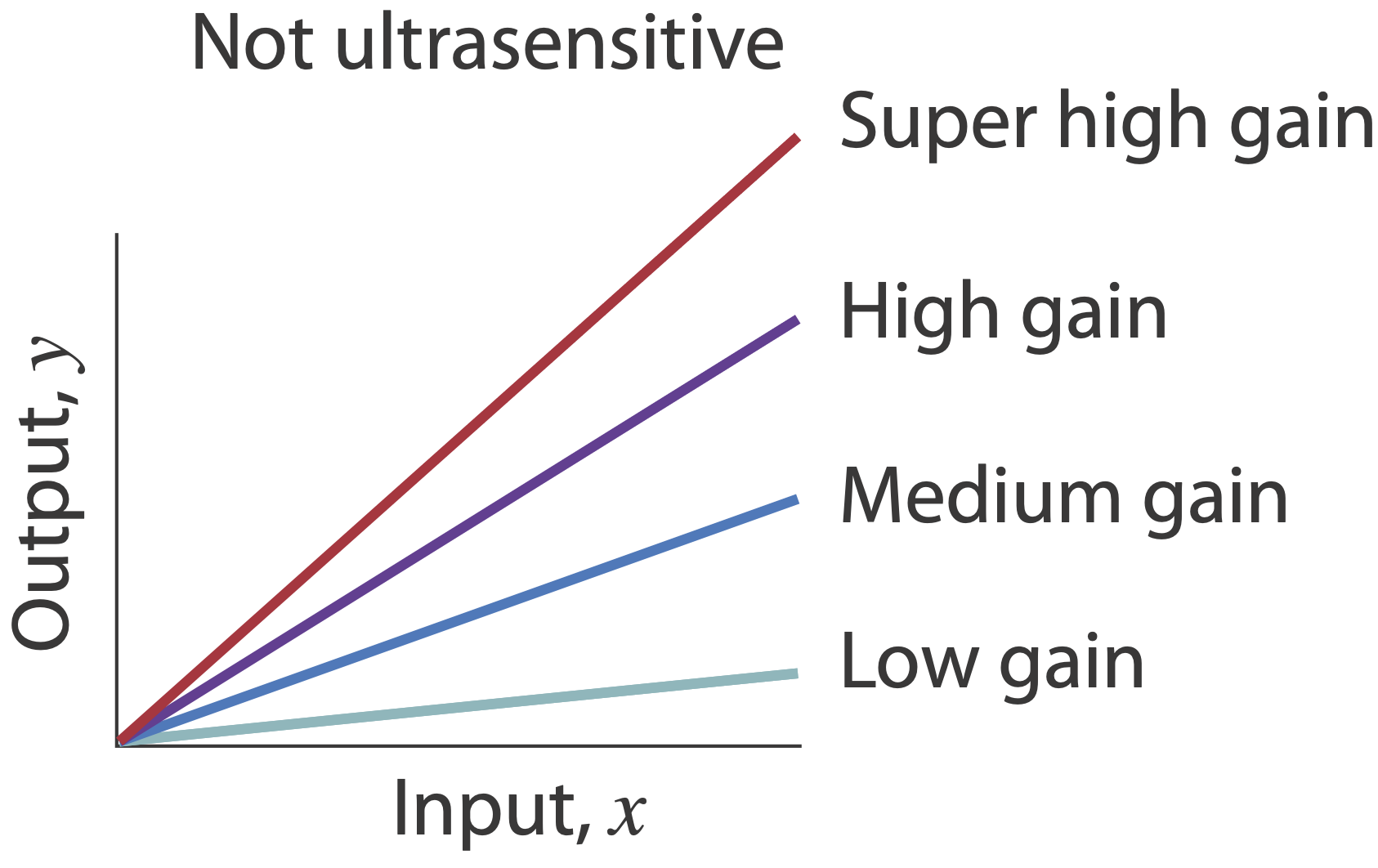
Ultrasensitivity is different than “gain.” A system in which $y = 100 x$ has very high gain, but is still responding linearly to its input, and is therefore not ultrasensitive.

Ultrasensitivity is necessary for many circuits - how can one generate it?¶

Ultrasensitivity plays a key role in many circuits. For example, together with positive feedback, it enables multistability. Together with negative feedback, it enables oscillations. Ultrasensitive can occur at different levels: for instance, in the transcriptional regulation of a target gene, or in the allosteric regulation of a protein. However, for many kinds of regulation that comprise circuits there is not necessarily a simple way to implement ultrasensitivity that does not require intricate engineering of cooperative molecular interactions.

Are there simple, generalizable, and engineerable design strategies that could confer ultrasensitivity Putting it another way, Suppose you need to create an ultrasensitive relationship between one species and its target. How would you do it?

For example, consider a simple gene regulatory system, in which an input activator, $A$, controls the expression of a target protein $Y$:

Let’s pause to ask:

How could you insert ultrasensitivity into the dependence of Y on A?
How could you make the threshold and sensitivity of the overall input function tunable?

Molecular titration “subtracts” one protein concentration from another.¶

Today we will discuss molecular titration, a simple and general mechanism that provides tunable ultrasensitivity across diverse natural systems, and allows engineering of ultrasensitive responses in synthetic circuits.

One of the most striking features of biological molecules is their ability to form strong and specific complexes with one another. Depending on the system, the complex itself may provide a particular activity, such as gene regulation. Or, alternatively, one of the monomers may provide an activity, with the complex inhibiting it.

In this example, molecular titration performs a kind of “subtraction” operation, in which an inhibitor (inactive species) “subtracts off” a fraction of otherwise active molecules.

Molecular titration occurs in diverse contexts:

In bacterial gene regulation, specialized transcription factors called sigma factors are stoichiometrically inhibited by cognate anti-sigma factors.
Transcription factors, such as basic helix-loop-helix proteins, form specific homo- and hetero-dimeric complexes with one another, each with a distinct binding specificity or activity.
Small RNA regulators can bind to cognate target mRNAs, inhibiting their translation.
Molecular circuits built out of nucleic acids must achieve ultrasensitivity using hybridization between complementary strands, an inherently 1:1 interaction. Molecular titration systems enable them to achieve high levels of ultrasensitivity, and thereby generate powerful dynamic behaviors.
In toxin-antitoxin systems, the “anti-toxin” protein can bind to its cognate toxin, blocking its activity. We already introduced the hipAB system and will talk more about it today.
Intercellular communication systems often work through direct complexes between ligands and receptors or ligands and inhibitors. In the next lecture we will consider the Notch signaling system, which involves tight stoichiometric interactions between Notch receptors and their ligands, such as Delta.

Today we will discuss the way in which these systems use molecular titration, through complex formation, to generate ultrasensitivity.

Molecular titration: a minimal model¶

To see how molecular titration produces ultrasensitivity we will consider the simplest possible example of two proteins, $A$ and $B$, that can bind to form a complex, $C$, that is inactive for both $A$ and $B$ activities. This system can be described by the following reactions:

\begin{align} A + B \underset{k_{\it{off}}}{\stackrel{k_\it{on}}{\rightleftharpoons}} C \end{align}

At steady-state, from mass action kinetics, we have:

\begin{align} k_\it{on} A B = k_\it{off} C \end{align}

Using $K_d = k_\it{off}/k_\it{on}$, we can write this as:

\begin{align} A B = K_d C. \end{align}

We also will insist on conservation of mass:

\begin{align} A_T &= A + C \\ B_T &= B + C \end{align}

Here, $A_T$ and $B_T$ denote the total amounts of $A$ and $B$, respectively. So, we have three equations and three unknowns, $A$, $B$, and $C$.

Solving these equations generates an expression for the amount of free $A$ or free $B$ as a function of $A_T$ and $B_T$ for different parameter values:

\begin{align} A = \frac{1}{2} \left( A_T-B_T-K_d+\sqrt{(A_T-B_T-K_d)^2+4A_T K_d} \right) \end{align}

What does this relationship look like? More specifically, let’s consider a case in which we control the total amount of $A_T$ and see how much free $A$ we get, for different amounts of $B_T$. We will start by assuming the limit of extremely strong binding (very values of $K_d$). And, we will plot this function on both linear and log-log scales:

[3]:

# array of A_total values
AT = np.linspace(0, 200, 1001)
Kd = 0.001
BTvals = np.array([50, 100, 150])

colors = bokeh.palettes.Blues3[::]

p = bokeh.plotting.figure(
    width=400,
    height=300,
    x_axis_label="A_T",
    y_axis_label="A",
    x_axis_type="linear",
    y_axis_type="linear",
    title="A vs. A_T",
    x_range=[AT.min(), AT.max()],
)

# Loop through colors and BT values (nditer not necessary)
A = np.zeros((BTvals.size, AT.size))
for i, (color, BT) in enumerate(zip(colors, BTvals)):
    A0 = 0.5 * (AT - BT - Kd + np.sqrt((AT - BT - Kd) ** 2 + 4 * AT * Kd))
    A[i, :] = A0
    p.line(AT, A0, line_width=2, color=color, legend_label=str(BT))

p.legend.location = "top_left"
p.legend.title = "B_T"
bokeh.io.show(p)

In these curves, we see that when $ A_T < B_T $, A is completely sequestered by B, and therefore close to 0. When $ A_T > B_T $, it rises linearly, becoming approximately proportional to the difference $A_T-B_T$. This is called a threshold-linear relationship. Plotting the same relationship on a log-log scale is also informative:

[4]:

# array of A_total values
AT = np.logspace(-2, 5, 1001)
Kd = 0.001
BTvals = np.logspace(-1, 3, 5)

# Decide on your color palette
colors = bokeh.palettes.Blues9[3:8][::-1]

p = bokeh.plotting.figure(
    width=450,
    height=300,
    x_axis_label="A_T",
    y_axis_label="A",
    x_axis_type="log",
    y_axis_type="log",
    title="A vs. A_T for different values of B_T, in strong binding regime, Kd<<1",
    x_range=[AT.min(), AT.max()],
)

# Loop through colors and BT values (nditer not necessary)
A = np.zeros((BTvals.size, AT.size))
for i, (color, BT) in enumerate(zip(colors, BTvals)):
    A0 = 0.5 * (AT - BT - Kd + np.sqrt((AT - BT - Kd) ** 2 + 4 * AT * Kd))
    A[i, :] = A0
    p.line(AT, A0, line_width=2, color=color, legend_label=str(BT))

p.legend.location = "bottom_right"
p.legend.title = "B_T"
bokeh.io.show(p)

The key feature to notice here is that A accumulates linearly at low and high values of $A_T$, but in between goes through a sharp transition, with a much higher slope, indicating ultrasensitivity, around $B_T$. Let’s plot the sensitivity as a function of $A_T$:

So far, we have looked in the “strong” binding limit, $K_d \ll 1$. But any real system will have a finite rate of unbinding. It is therefore important to see how the system behaves across a range of $K_d$ values.

[5]:

# array of A_total values
AT = np.logspace(-2, 3, 1001)
BT = 1
Kdvals = np.logspace(-3, 1, 5)

# Decide on your color palette
colors = bokeh.palettes.Blues9[3:8][::-1]

p = bokeh.plotting.figure(
    width=400,
    height=300,
    x_axis_label="A_T",
    y_axis_label="A",
    x_axis_type="log",
    y_axis_type="log",
    title="A vs. A_T for different values of Kd, B_T=1",
    x_range=[AT.min(), AT.max()],
)


# Loop through colors and BT values (nditer not necessary)
A = np.zeros((Kdvals.size, AT.size))
for i, (color, Kd) in enumerate(zip(colors, Kdvals)):
    A0 = 0.5 * (AT - BT - Kd + np.sqrt((AT - BT - Kd) ** 2 + 4 * AT * Kd))
    A[i, :] = A0
    p.line(AT, A0, line_width=2, color=color, legend_label=str(Kd))

p.legend.location = "bottom_right"
p.legend.title = "K_d"
bokeh.io.show(p)

Here we see that the tighter the binding, the more completely $B$ shuts off $A$, and the larger the region of ultrasensitivity around the transition point.

On a linear scale, zooming in around the transition point, we can see that weaker binding “softens” the transition from flat to linear behavior:

[6]:

# array of A_total values
AT = np.linspace(50, 150, 1001)
Kdvals = np.array([0.01, 0.1, 0.5, 1])
BT = 100

colors = bokeh.palettes.Blues8[::]

p = bokeh.plotting.figure(
    width=400,
    height=300,
    x_axis_label="A_T",
    y_axis_label="A",
    x_axis_type="linear",
    y_axis_type="linear",
    title="A vs. A_T for different K_d values",
    x_range=[AT.min(), AT.max()],
)

# Loop through colors and BT values (nditer not necessary)
A = np.zeros((Kdvals.size, AT.size))
for i, (color, Kd) in enumerate(zip(colors, Kdvals)):
    A0 = 0.5 * (AT - BT - Kd + np.sqrt((AT - BT - Kd) ** 2 + 4 * AT * Kd))
    A[i, :] = A0
    p.line(AT, A0, line_width=2, color=color, legend_label=str(Kd))

p.legend.location = "top_left"
p.legend.title = "Kd"
bokeh.io.show(p)

Ultrasensitivity in threshold-linear response functions¶

Threshold-linear responses differ qualitatively from what we had with a Hill function. Unlike the sigmoidal, or “S-shaped,” Hill function, which saturates at a maximum “ceiling,” the threshold-linear function increases without bound, maintaining a constant slope as input values increase.

Despite these differences, we can still quantify the sensitivity of this response. A simple way to define sensitivity is the fold change in output for a given fold change in input, evaluated at a particular operating point. The plots below show this sensitivity, $S=\frac{d log A}{d log A_T}$ plotted for varying $A_T$, and for different values of $K_d$. Note the peak in $S$ right around the transition, whose strength grows with tighter binding (lower $K_d$). This peak is just highlighting what we can already see in the input-output: ultrasensitivity can be very strong in the neighborhood of the

[7]:

# array of A_total values, base 2
AT = np.logspace(-5, 5, 1001, base=2)
Kdvals = np.array([0.00001, 0.0001, 0.001, 0.01, 0.1])
BT = 1

# Color palettes:
colors = bokeh.palettes.Blues9[:][::]
scolors = bokeh.palettes.Oranges9[:][::]

pA = bokeh.plotting.figure(
    width=300,
    height=200,
    x_axis_label="A_T",
    y_axis_label="A",
    x_axis_type="log",
    y_axis_type="log",
    title="A vs A_T for several K_d",
    x_range=[AT.min(), AT.max()],
)

pS = bokeh.plotting.figure(
    width=300,
    height=200,
    x_axis_label="A_T",
    y_axis_label="S",
    x_axis_type="log",
    y_axis_type="log",
    title="Sensitivity vs. A_T for several K_d",
    x_range=[AT.min(), AT.max()],
)

# Loop through colors and BT values (nditer not necessary)
A = np.zeros((Kdvals.size, AT.size))  # store A values
S = np.zeros(
    (Kdvals.size, AT.size - 1)
)  # sensitivities are derivatives, so there is one fewer of them
foldstep = AT[1] / AT[0]
for i, (color, scolor, Kd) in enumerate(zip(colors, scolors, Kdvals)):
    A0 = 0.5 * (AT - BT - Kd + np.sqrt((AT - BT - Kd) ** 2 + 4 * AT * Kd))
    A[i, :] = A0
    pA.line(AT, A0, line_width=2, color=color, legend_label=str(Kd))

    # define Sensitivity, S, as dlog(A)/dlog(AT)=AT/A*dA/d(AT)
    S0 = (
        AT[0:-2]
        / A[i, 0:-2]
        * (A[i, 1:-1] - A[i, 0:-2])
        / (AT[1:-1] - AT[0:-2])
    )
    pS.line(AT[0:-2], S0, line_width=2, color=scolor, legend_label=str(Kd))

pA.legend.location = "bottom_right"
pA.legend.title = "Kd"
pS.legend.location = "bottom_right"
pS.legend.title = "Kd"

bokeh.io.show(bokeh.layouts.gridplot([pA, pS], ncols=2))

Incorporating production and degradation¶

So far, we considered a static pool of $A$ and $B$, but in a cell, both proteins undergo continuous synthesis as well as degradation and/or dilution. Representing these dynamics explicitly leads to similar ultrasensitive responses, but now in terms of the protein production and degradation rates (see Buchler and Louis, JMB 2008):

\begin{align} \frac{dA}{dt}&=\beta_A - k_{on} A B + k_{\it{off}} C - \gamma_A A \\ \frac{dB}{dt}&=\beta_B - k_{on} A B + k_{\it{off}} C - \gamma_B B \\ \frac{dC}{dt}&= k_{on} A B - k_\it{off} C - \gamma_C C \\ \end{align}

Here, we assume a distinct decay rate for $C$, but we could alternatively consider degradation of its $A$ and $B$ constituents at their normal rates.

Demonstrating titration synthetically¶

Simple models like the ones above can help us think about what behaviors we should expect in a system. But how do we know if they accurately describe the real behavior of a complex molecular system, particularly one operating in the even more complex milieu of the living cell?

To find out, Buchler and Cross used a synthetic biology approach to test whether this simple scheme could indeed generate the predicted ultrasensitivity.

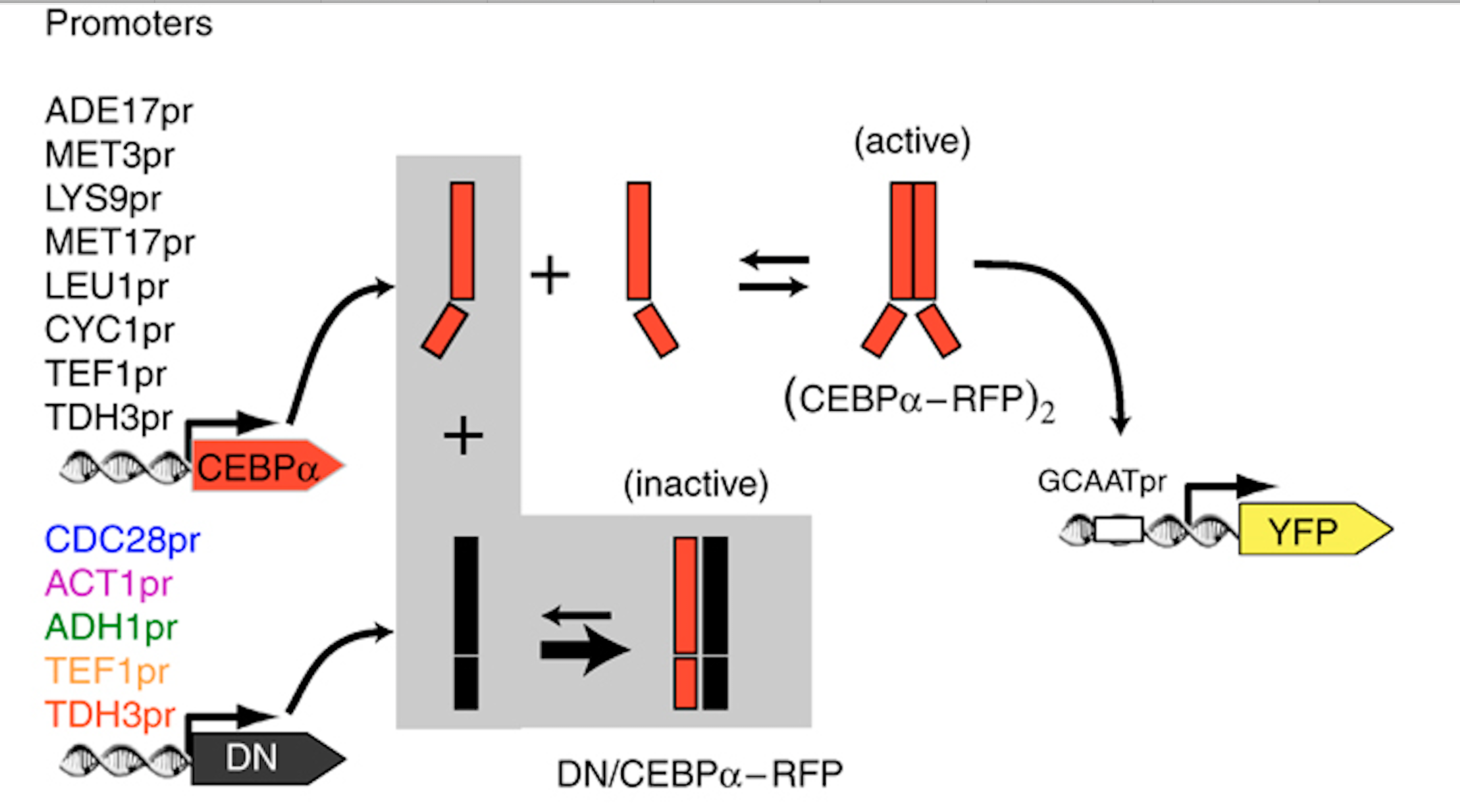
They engineered yeast cells to express a transcription factor, a stoichiometric inhibitor of that factor, and a target reporter gene to readout the level of the transcription factor. As an activator they used the mammalian bZip family activator CEBP/$\alpha$. As the inhibitor they used a previously identified dominant negative mutant that binds to CEBP/$\alpha$ with a tight $K_d \approx 0.04 nM$. As a reporter they used a yellow fluorescent protein. To vary the relative levels of the activator and inhibitor, they expressed them from promoters of different strengths, which are listed in the column on the left of the figure. As a control, they also constructed yeast strains without the inhibitor.

The scheme is shown here:

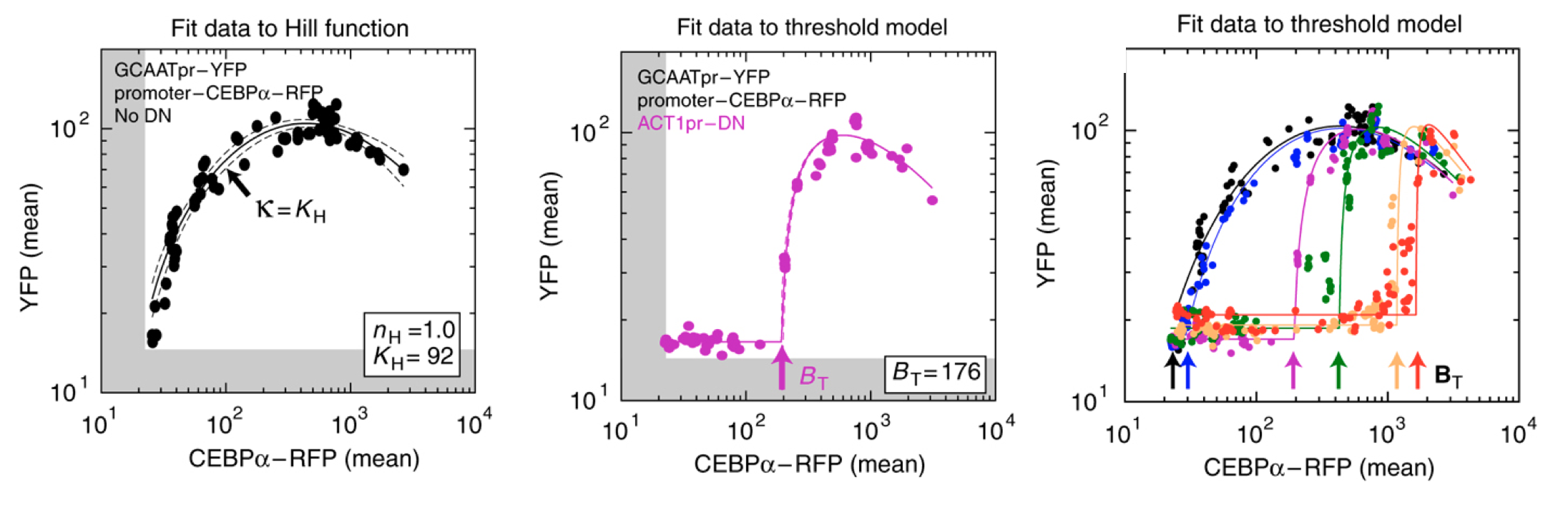
As shown below (left), the activator generated a dose-dependent increase in the fluorescent protein. (The noticeable decrease at the highest levels is attributed to the interesting effect of transcriptional “squelching”–see paper for details).

Adding the inhibitor (middle panel) produced the predicted threshold-linear response.

Finally, expressing the inhibitor from promoters of different strengths (right) showed corresponding shifts in the threshold position, as expected based on their independently measured expression levels (not shown).

The conclusions so far:

Tight binding can produce ultrasensitivity through molecular titration.
Molecular titration is a real effect that can be reconstituted and quantitatively predicted in living cells.

We now turn to biological contexts in which molecular titration appears.

small RNA regulation can generate ultrasensitive responses through molecular titration¶

One of the most stunning discoveries of the last several decades is the pervasive and diverse roles that small RNA molecules play in regulating gene expression, from bacteria to mammalian cells. micro RNA (miRNA) represents a major class of regulatory RNA molecules in eukaryotes. Individual miRNAs typically target hundreds of genes. Conversely, most protein-coding genes are miRNA targets. miRNAs can be highly expressed (as much as 50,000 copies per cell).

Many miRNAs exhibit strong sequence conservation across species, suggesting selection for function.

Confusingly, however, at the cell population average level, they sometimes appear to generate relatively weak repression.

To more quantitatively understand how miRNA regulation operates, Mukherji et al developed a system to analyze miRNA regulation at the level of single cells (Mukherji, S., et al, Nat. Methods, 2011).

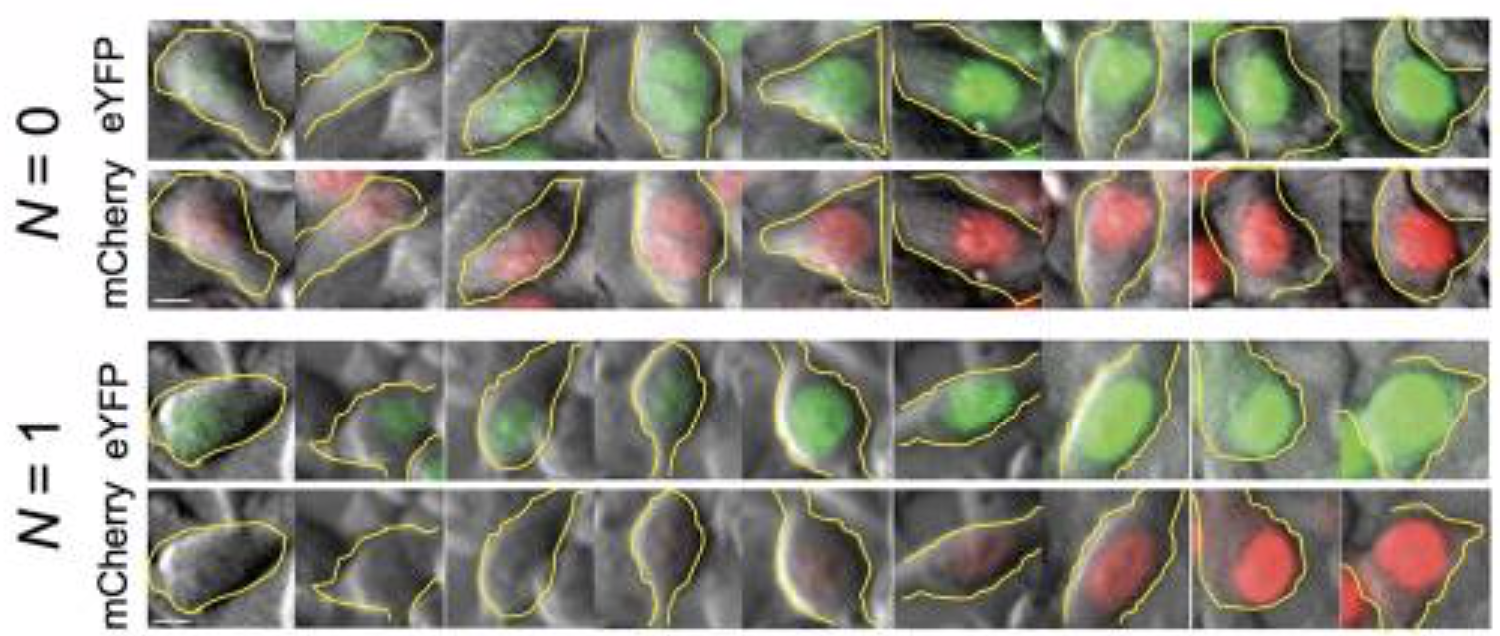
The key idea of the design is to express two distinguishable fluorescent proteins, one of which is regulated by a specific miRNA, with the other serving as an unregulated internal control.

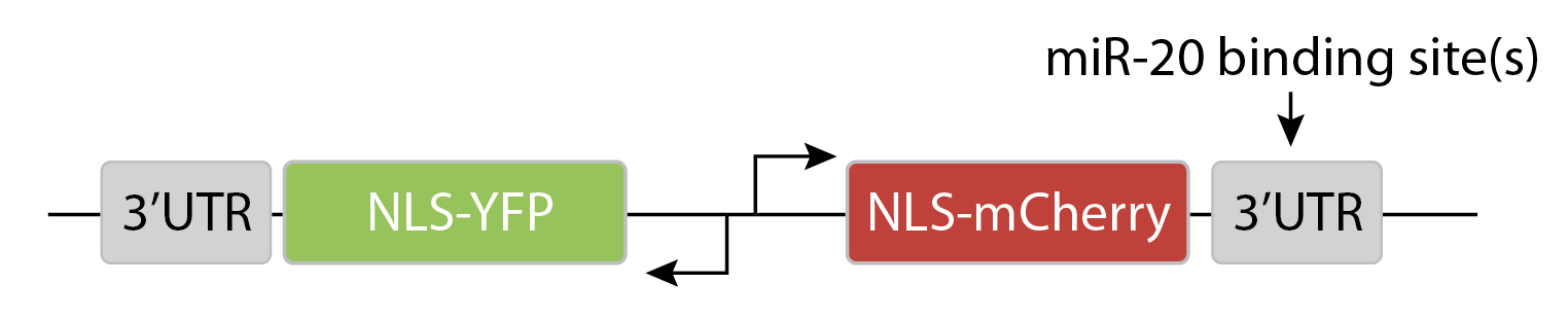
They transfected variants of this construct with (N=1) or without (N=0) a binding site for the miR-20 miRNA. The images below show the levels of the two proteins in different individual cells, sorted by their intensity. The top pair of rows shows the case with no miRNA binding sites, and the lower pair of rows shows the case with binding sites. Without the binding site, the two colors appear to be proportional to each other, as you would expect, since they are co-regulated. On the other hand, with the binding site, mCherry expression is suppressed at lower YFP expression levels. Only at the higher YFP levels do you start to see the mCherry signal growing.

This can be seen more clearly in a scatter plot of the two colors:

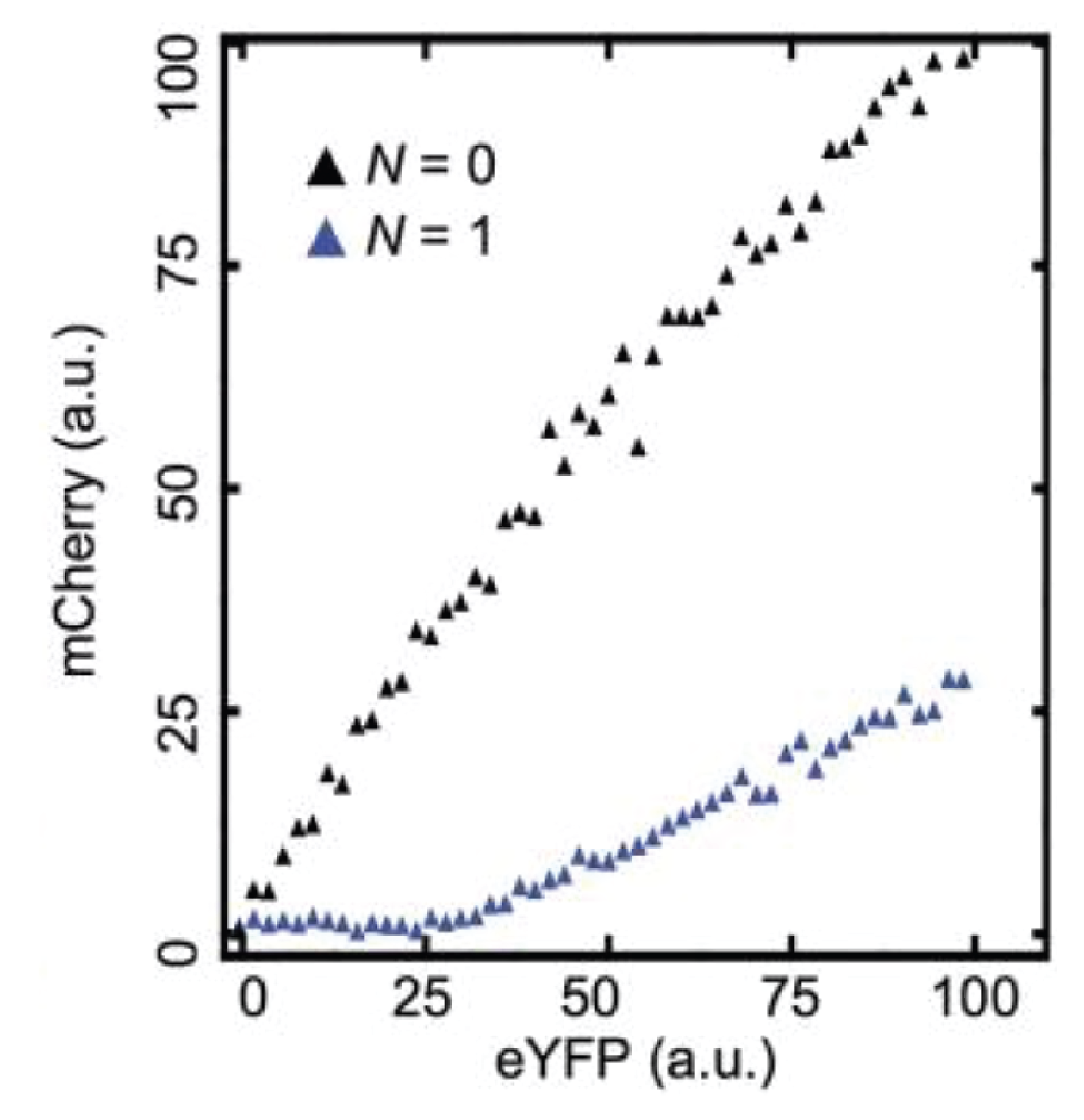
Here, the YFP x-axis is analogous to our $A_T$, above, while the mCherry y-axis is analogous to $A$.

The authors go on to explore how increasing the number of binding sites can modulate the threshold for repression. The results broadly fit the behavior expected from the molecular titration model.

These results could help reconcile the very different types of effects one sees for miRNAs in different contexts. Sometimes they appear to provide strong, switch-like effects, as with fate-controlling miRNAs in C. elegans. On the other hand, in many other contexts, they appear to exert much weaker “fine-tuning” effects on their targets.

That makes sense: when miRNAs are unsaturated, they can have a relatively strong effect on their target expression levels, essentially keeping them “off.” On the other hand, when targets are expressed highly enough, the relative effect of the miRNA on expression becomes much weaker, effectively just shifting it to slightly slower values.

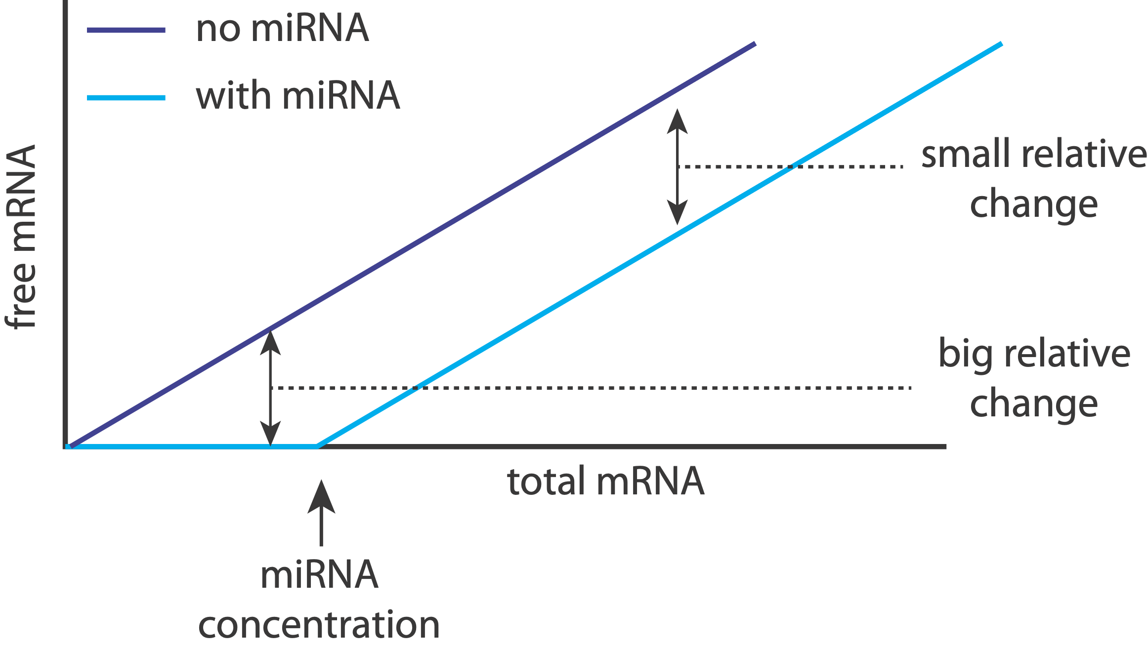
Returning to the question posed earlier, we now see that a remarkably simple way to create a threshold within a regulatory step is to insert a constitutive, inhibitory miRNA:

Note that in addition to its general regulatory abilities and thresholding effects, miRNA regulation can also reduce noise in target gene expression. See Schmiedel et al, “MicroRNA control of protein expression noise,” Science (2015).

Molecular titration in antibiotic persistence¶

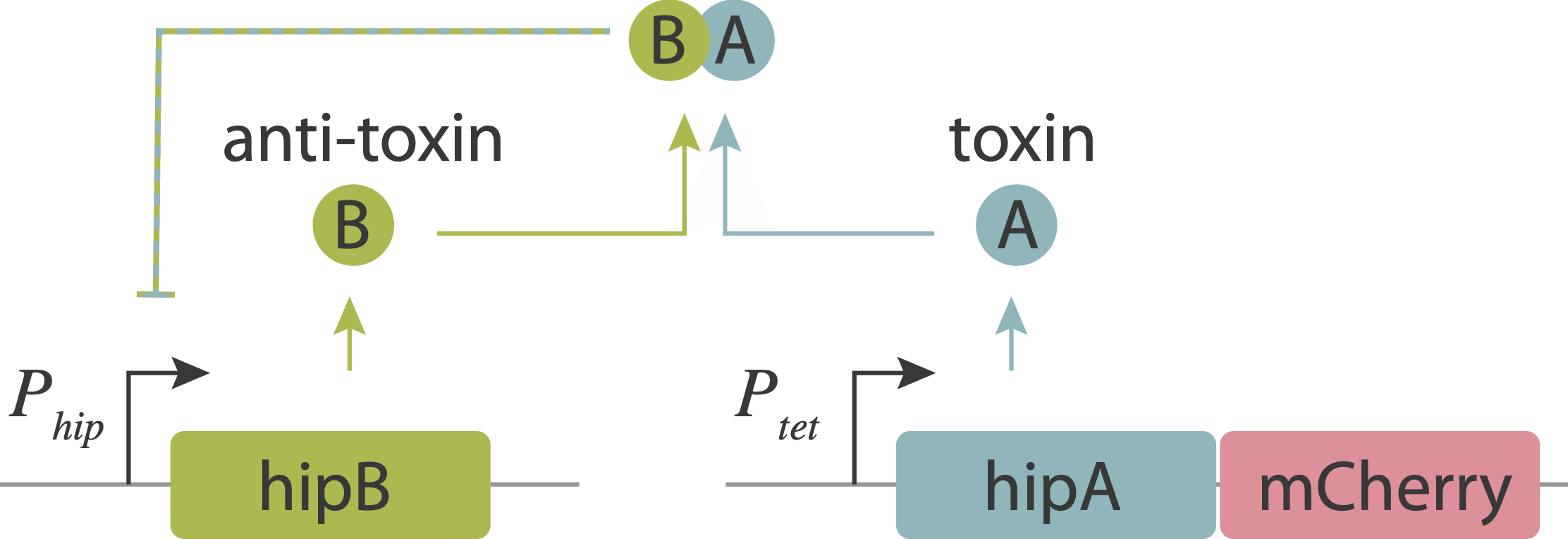
Now, let’s return to the persistence circuit that we introduced in the bet-hedging lecture. As you recall, beautiful imaging studies, combining microfluidic devices with time-lapse imaging revealed that individual bacteria stochastically enter slow-growing persistent states that tolerate antibiotics, and do so even in the absence of those antibiotics. The hipAB circuit generates such episodes. It comprises a toxin protein, HipA, and a cognate anti-toxin, HipB. The two proteins are expressed from a single operon. They form tight complexes that also act to repress their own promoter. Entry into persistent states could occur from stochastic noise, which allows the levels of the HipA toxin to occasionally exceed those of the HipB anti-toxin. Thus, the hipAB circuit combines three key design features that we have studied in this course: noise, negative autoregulation, and molecular titration.

The hipAB toxin-antitoxin circuit

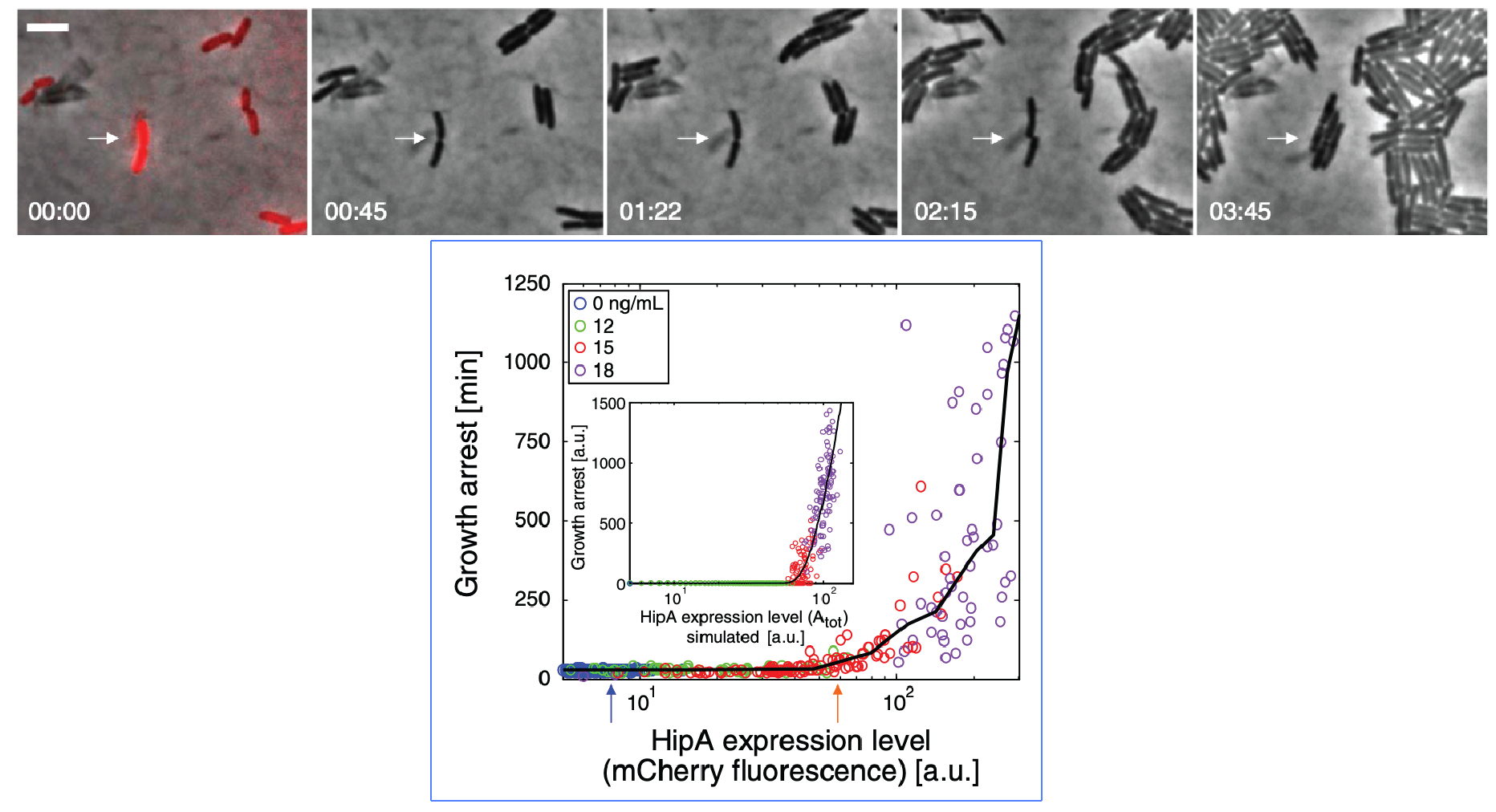
Evidence that molecular titration plays a key role in activation of persistence was shown by Rotem et al. Among many experiments, they created a partial open loop strain in which they could independently control hipA and read its level out in individual cells using a co-transcribed red fluorescent protein (mCherry):

hipAB_partial_open_loop

They then used time-lapse movies to correlate the growth behavior of individual cells with their HipA protein levels. As shown in these panels, cells with higher levels of mCherry showed delayed growth. Analyzing these data quantitatively revealed (drumroll, please) a threshold relationship, in which growth arrest occurred when HipA (as measured by its fluorescent protein tag) exceeded a threshold concentration:

persister_mCherry

Note that the inset in the plot is the behavior of a mathematical model of the circuit.

A molecular titration circuit explains persistence.¶

The experimental results strongly suggest the possibility that hipA-hipB could allow stochastic initiation of persistence by taking advantage of the ultrasensitivity of protein-level molecular titration. Here we will use a model to understand the dynamics that this circuit could generate.

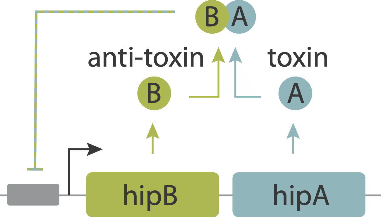
Here, we implement the model of Koh and Dunlop (BMC Syst. Biol., 2012). The circuit is shown in the image below, taken from the paper.

Dunlop hipAB circuit

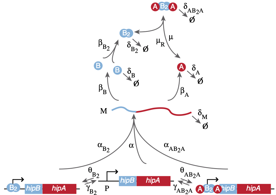
Two genes, the toxin hipA and an antitoxin hipB are under control of the same promoter. HipB can form a homodimer, and that dimer can be further complexed with two HipA molecules to form a complex. This complex, and also the HipB dimers, may bind the promoter and repress expression. Noise is essential for the operation of this circuit. If we analyze it deterministically, it will always produce an excess of anti-toxin over toxin, and never do anything interesting! Therefore, we will use the Gillespie stochastic simulation algorithm to explore its behavior with noise.

As with any Gillespie simulation, it is best to make a table that lists all molecular species, the reactions or transitions they are allowed to participate in, and their corresponding propensities. We also create a table of parameter values.

First, we’ll start with the species, bearing in mind that the promoter can exist in three states: bare, bound with HipB dimer, and bound with the HipA/HipB complex.

index	description	variable
0	mRNA copy number	`m`
1	HipA copy number	`a`
2	HipB copy number	`b`
3	Dimerized HipB copy number	`b2`
4	HipA/HipB complex copy number	`ab2a`
5	unbound promoter copy number	`p`
6	promoter bound to HipB dimer copy number	`pb2`
7	promoter bound to HipA/HipB copy number	`pab2a`

With the species defined, we can write the move set with propensities. We base each allowed transition on the diagram of the circuit, above.

index	description	update	propensity
0	production of mRNA from unbound promoter	`m ⟶ m + 1`	`alpha * p`
1	production of mRNA from promoter with HipB bound	`m ⟶ m + 1`	`alpha_b2 * pb2`
2	production of mRNA from promoter with complex bound	`m ⟶ m + 1`	`alpha_ab2a * pab2a`
3	production of HipA monomer	`a ⟶ a + 1`	`beta_a * m`
4	production of HipB monomer	`b ⟶ b + 1`	`beta_b * m`
5	HipB dimerization	`b ⟶ b - 2`, `b2 ⟶ b2 + 1`	`beta_b2 * b * (b-1)`
6	HipA/HipB complex formation	`b2 ⟶ b2 - 1`, `ab2a ⟶ ab2a + 1`, `a ⟶ a - 2`	`mu * b2 * a * (a-1)`
7	binding of HipB dimer to promoter	`p ⟶ p - 1`, `pb2 ⟶ pb2 + 1`, `b2 ⟶ b2 - 1`	`theta_b2 * p * b2`
8	binding of HipA/HipB complex to promoter	`p ⟶ p - 1`, `pab2a ⟶ pab2a + 1`, `ab2a ⟶ ab2a - 1`	`theta_ab2a * p * ab2a`
9	degradation of mRNA	`m ⟶ m - 1`	`delta_m * m`
10	degradation of HipA monomer	`a ⟶ a - 1`	`delta_a * a`
11	degradation of HipB monomer	`b ⟶ b - 1`	`delta_b * b`
12	degradation of HipB dimer	`b2 ⟶ b2 - 1`	`delta_b2 * b2`
13	degradation of HipA/HipB complex	`ab2a ⟶ ab2a - 1`	`delta_ab2a * ab2a`
14	dissociation of HipA/HipB complex	`b2 ⟶ b2 + 1`, `ab2a ⟶ ab2a - 1`, `a ⟶ a + 2`	`mu_r * ab2a`
15	dissociation of HipB dimer from promoter	`p ⟶ p + 1`, `pb2 ⟶ pb2 - 1`, `b2 ⟶ b2 + 1`	`gamma_b2 * pb2`
16	dissociation of HipA/HipB complex from promoter	`p ⟶ p + 1`, `pab2a ⟶ pab2a - 1`, `ab2a ⟶ ab2a + 1`	`gamma_ab2a * pab2a`

Finally, we can write parameter values, taken from the Koh and Dunlop paper.

parameter	value	units
`alpha`	60	1/h
`alpha_b2`	6	1/h
`alpha_ab2a`	6	1/h
`beta_a`	12	1/h
`beta_b`	60	1/h
`beta_b2`	60	1/h
`mu`	60	1/h
`theta_b2`	1500	1/h
`theta_ab2a`	1500	1/h
`delta_m`	6	1/h
`delta_a`	1.2	1/h
`delta_b`	18	1/h
`delta_b2`	5	1/h
`delta_ab2a`	1.2	1/h
`mu_r`	60	1/h
`gamma_b2`	60	1/h
`gamma_ab2a`	60	1/h

These tables define the species and transition rates, and therefore the master equation, and therefore also the simulation. So, it is a matter of coding it up from the tables. We’ll start with the propensity function.

[8]:

@numba.njit
def propensity(
    propensities,
    population,
    t,
    alpha,
    alpha_b2,
    alpha_ab2a,
    beta_a,
    beta_b,
    beta_b2,
    mu,
    theta_b2,
    theta_ab2a,
    delta_m,
    delta_a,
    delta_b,
    delta_b2,
    delta_ab2a,
    mu_r,
    gamma_b2,
    gamma_ab2a,
):
    m, a, b, b2, ab2a, p, pb2, pab2a = population

    propensities[0] = alpha * p
    propensities[1] = alpha_b2 * pb2
    propensities[2] = alpha_ab2a * pab2a
    propensities[3] = beta_a * m
    propensities[4] = beta_b * m
    propensities[5] = beta_b2 * b * (b - 1)
    propensities[6] = mu * b2 * a * (a - 1)
    propensities[7] = theta_b2 * p * b2
    propensities[8] = theta_ab2a * p * ab2a
    propensities[9] = delta_m * m
    propensities[10] = delta_a * a
    propensities[11] = delta_b * b
    propensities[12] = delta_b2 * b2
    propensities[13] = delta_ab2a * ab2a
    propensities[14] = mu_r * ab2a
    propensities[15] = gamma_b2 * pb2
    propensities[16] = gamma_ab2a * pab2a

And now we can build the update matrix for the respective species, each line representing the corresponding reaction:

[9]:

update = np.array(
    [   # m   a   b  b2 ab2a  p pb2 pab2a
        # 0   1   2   3   4   5   6   7
        [ 1,  0,  0,  0,  0,  0,  0,  0],  # 0
        [ 1,  0,  0,  0,  0,  0,  0,  0],  # 1
        [ 1,  0,  0,  0,  0,  0,  0,  0],  # 2
        [ 0,  1,  0,  0,  0,  0,  0,  0],  # 3
        [ 0,  0,  1,  0,  0,  0,  0,  0],  # 4
        [ 0,  0, -2,  1,  0,  0,  0,  0],  # 5
        [ 0, -2,  0, -1,  1,  0,  0,  0],  # 6
        [ 0,  0,  0, -1,  0, -1,  1,  0],  # 7
        [ 0,  0,  0,  0, -1, -1,  0,  1],  # 8
        [-1,  0,  0,  0,  0,  0,  0,  0],  # 9
        [ 0, -1,  0,  0,  0,  0,  0,  0],  # 10
        [ 0,  0, -1,  0,  0,  0,  0,  0],  # 11
        [ 0,  0,  0, -1,  0,  0,  0,  0],  # 12
        [ 0,  0,  0,  0, -1,  0,  0,  0],  # 13
        [ 0,  2,  0,  1, -1,  0,  0,  0],  # 14
        [ 0,  0,  0,  1,  0,  1, -1,  0],  # 15
        [ 0,  0,  0,  0,  1,  1,  0, -1],  # 16
    ],
    dtype=int,
)

For convenience, we will again store the parameters in a NamedTuple to enable easy access.

[10]:

ParametersSSA = collections.namedtuple(
    "ParametersSSA",
    [
        "alpha",
        "alpha_b2",
        "alpha_ab2a",
        "beta_a",
        "beta_b",
        "beta_b2",
        "mu",
        "theta_b2",
        "theta_ab2a",
        "delta_m",
        "delta_a",
        "delta_b",
        "delta_b2",
        "delta_ab2a",
        "mu_r",
        "gamma_b2",
        "gamma_ab2a",
    ],
)

params_ssa = ParametersSSA(
    alpha=60,
    alpha_b2=6,
    alpha_ab2a=6,
    beta_a=12,
    beta_b=60,
    beta_b2=60,
    mu=60,
    theta_b2=1500,
    theta_ab2a=1500,
    delta_m=6,
    delta_a=1.2,
    delta_b=18,
    delta_b2=5,
    delta_ab2a=1.2,
    mu_r=60,
    gamma_b2=60,
    gamma_ab2a=60,
)

Next, we can specify the initial condition, as well as the time points we wish to evaluate in the simulation. For our initial condition, we will have no species at all, except for one bare promoter. We will start by simulating for 24 hours.

[11]:

population_0 = np.array([0, 0, 0, 0, 0, 1, 0, 0], dtype=int)
time_points = np.linspace(0, 44, 800)

We will make an adjustment to the parameters as given in the Koh and Dunlop paper. We will instead accelerate the degradation of the toxin.

Now we can perform the simulation.

[12]:

# Perform the Gillespie simulation
pop = biocircuits.gillespie_ssa(
    propensity, update, population_0, time_points, args=tuple(params_ssa)
)

To parse the results, we would like to have the total HipA and HipB concentrations. Furthermore, following Koh and Dunlop, we define a ratio $R$ to be the amount of HipA monomer divided by the total amount of noncomplexed HipA and HipB (including HipA monomers, HipB monomers, and HipB dimers).

[13]:

# Extract HipA and HipB concs
total_hipA = pop[0, :, 1] + pop[0, :, 4] * 2 + pop[0, :, 7] * 2
total_hipB = (
    pop[0, :, 2]
    + pop[0, :, 3] * 2
    + pop[0, :, 4] * 2
    + pop[0, :, 6] * 2
    + pop[0, :, 7] * 2
)

# Compute R
R = np.empty(len(time_points))
inds = pop[0, :, 1] > 0
R[~inds] = 0.0
R[inds] = pop[0, inds, 1] / (
    pop[0, inds, 1] + pop[0, inds, 2] + pop[0, inds, 3] * 2
)

Finally, we can plot the results. Actually, instead of plotting them directly, we will build a dashboard so that we can vary parameters and see how things change. (This does make the preceding cells unnecessary, but we showed those steps for clarity.)

[14]:

# Set up parameter input as text boxes
params_txt = [
    pn.widgets.TextInput(name=key, value=str(val))
    for key, val in params_ssa._asdict().items()
]

params_txt.append(pn.widgets.TextInput(name="time", value="50"))
params_txt.append(pn.widgets.TextInput(name="# of time points", value="1000"))

deps = tuple([params_txt[i].param.value for i in range(len(params_txt))])


@pn.depends(*deps)
def plots(
    alpha,
    alpha_b2,
    alpha_ab2a,
    beta_a,
    beta_b,
    beta_b2,
    mu,
    theta_b2,
    theta_ab2a,
    delta_m,
    delta_a,
    delta_b,
    delta_b2,
    delta_ab2a,
    mu_r,
    gamma_b2,
    gamma_ab2a,
    time_end,
    n_time_points,
):

    params = ParametersSSA(
        alpha=float(alpha),
        alpha_b2=float(alpha_b2),
        alpha_ab2a=float(alpha_ab2a),
        beta_a=float(beta_a),
        beta_b=float(beta_b),
        beta_b2=float(beta_b2),
        mu=float(mu),
        theta_b2=float(theta_b2),
        theta_ab2a=float(theta_ab2a),
        delta_m=float(delta_m),
        delta_a=float(delta_a),
        delta_b=float(delta_b),
        delta_b2=float(delta_b2),
        delta_ab2a=float(delta_ab2a),
        mu_r=float(mu_r),
        gamma_b2=float(gamma_b2),
        gamma_ab2a=float(gamma_ab2a),
    )

    time_points = np.linspace(0, float(time_end), int(n_time_points))

    pop = biocircuits.gillespie_ssa(
        propensity, update, population_0, time_points, args=tuple(params)
    )

    # Extract HipA and HipB concs
    total_hipA = pop[0, :, 1] + pop[0, :, 4] * 2 + pop[0, :, 7] * 2
    total_hipB = (
        pop[0, :, 2]
        + pop[0, :, 3] * 2
        + pop[0, :, 4] * 2
        + pop[0, :, 6] * 2
        + pop[0, :, 7] * 2
    )

    # Compute R
    R = np.empty(len(time_points))
    inds = pop[0, :, 1] > 0
    R[~inds] = 0.0
    R[inds] = pop[0, inds, 1] / (
        pop[0, inds, 1] + pop[0, inds, 2] + pop[0, inds, 3] * 2
    )

    # Mean levels
    mean_A = pop[0, :, 1].mean()
    mean_B = (pop[0, :, 1] + pop[0, :, 2] + pop[0, :, 3] * 2).mean()

    p = bokeh.plotting.figure(
        frame_width=550,
        frame_height=200,
        x_axis_label="time (h)",
        y_axis_label="copies",
        x_range=[0, time_points[-1]],
        title="mean free HipA: {0:.1f}; mean free HipB: {1:.1f}".format(
            mean_A, mean_B
        ),
    )
    p.line(time_points, total_hipB, line_join="bevel", legend_label="HipB")
    p.line(
        time_points,
        total_hipA,
        line_color="tomato",
        line_join="bevel",
        legend_label="HipA",
    )

    # Plot of ratio
    p2 = bokeh.plotting.figure(
        frame_width=550,
        frame_height=200,
        x_axis_label="time (h)",
        y_axis_label="R",
    )
    p2.line(time_points, R, line_join="bevel", color="black")

    # Lock the x_ranges
    p2.x_range = p.x_range

    return bokeh.layouts.column([p, p2])


# Build the widgets
widgets = pn.Row(
    *tuple(
        [
            pn.Column(
                *tuple(
                    params_txt[
                        i
                        * len(params_txt)
                        // 9 : (i + 1)
                        * len(params_txt)
                        // 9
                    ]
                ),
                width=75
            )
            for i in range(9)
        ]
    )
)

pn.Column(plots, pn.Spacer(height=15), widgets)

Data type cannot be displayed:

[14]:

We see that HipA and HipB closely track each other, as we would expect since they are under control of the same promoter. On rare occasions, $R > 1/2$, meaning that there is more toxin than antitoxin, which could lead to persistence.

To see how often a the cell is persistent, we can compute the fraction of time it is persistent. We will run a very long calculation and tally up how often is it persistent, that is with $R > 1/2$. (We could do this more accurately with event handling in the simulation, but this will suffice for our purposes.)

[15]:

time_points = np.linspace(0, 1000, 50000)

# Perform the Gillespie simulation
pop = biocircuits.gillespie_ssa(
    propensity, update, population_0, time_points, args=tuple(params_ssa)
)

# Extract HipA and HipB concs
total_hipA = pop[0, :, 1] + pop[0, :, 4] * 2 + pop[0, :, 7] * 2
total_hipB = (
    pop[0, :, 2]
    + pop[0, :, 3] * 2
    + pop[0, :, 4] * 2
    + pop[0, :, 6] * 2
    + pop[0, :, 7] * 2
)

# Compute R
R = np.empty(len(time_points))
inds = pop[0, :, 1] > 0
R[~inds] = 0.0
R[inds] = pop[0, inds, 1] / (
    pop[0, inds, 1] + pop[0, inds, 2] + pop[0, inds, 3] * 2
)

# Only look at steady state
R = R[len(R) // 2 :]

print("Fraction of time competent: {0:.4f}".format((R > 0.5).sum() / len(R)))

Fraction of time competent: 0.0695

The cells are competent nearly 10% of the time with these parameters. This is a bit high, and the time that they are competent can by controlled by varying the parameters.

Beyond pairwise titration¶

Today we talked about molecular titration arising from interactions between protein pairs. However, proteins often form more complex, and even combinatorial, networks of homo- and hetero-dimerizing components. One example occurs in the control of cell death (apoptosis) by Bcl2-family proteins, a process that naturally should be performed in an all-or-none way. Another example that we will discuss soon involves the formation of signaling complexes in promiscuous ligand-receptor systems.

Conclusions¶

Today we have seen that molecular titration provides a simple but powerful way to generate ultrasensitive responses across different types of molecular systems:

The general principle of molecular titration: formation of a tight complex between two species makes the concentration of a “free” protein species depend in a threshold-linear manner on its total level or rate of production.
Molecular titration could explain key features of miRNA based regulation.
Molecular titration appears to underlie the generation of bacterial persisters through toxin-antitoxin systems.
Molecular titration between co-expressed, mutually inhibitory ligands and receptors can generate exclusive send-or-receive signaling states in the Notch signaling pathway.

Computing environment¶

[16]:

%load_ext watermark
%watermark -v -p numpy,scipy,numba,biocircuits,bokeh,panel,jupyterlab

CPython 3.7.7
IPython 7.13.0

numpy 1.18.1
scipy 1.4.1
numba 0.49.0
biocircuits 0.0.17
bokeh 2.0.2
panel 0.9.5
jupyterlab 1.2.6