9. Oscillators, part II: Uses, simplifications, and elaborations of negative feedback oscillators
Design principles
Oscillator phase can be used as a growth timer.
Ultrasensitive delayed repression produces oscillations in gene expression.
Combination of delayed negative feedback with positive feedback enables independent tuning of oscillator period and amplitude.
Techniques
Linear stability analysis of delay differential equations (DDEs)
“Brute force” linear stability diagrams
Numerical solution of DDEs
[1]:
import numpy as np
import scipy.integrate
import scipy.interpolate
import scipy.optimize

import bokeh.io
import bokeh.plotting

bokeh.io.output_notebook()
The repressilator, introduced in the previous lecture, shows that delayed negative feedback, under the right conditions, can provide robust oscillations. Today, we will further explore this circuit design, showing how it can be used as a timer to record bacterial growth in the mammalian gut, simplified into a single gene oscillator, and extended with the addition of positive feedback to allow independent tuning of period and amplitude.
Part I: Precision repressilators can record bacterial growth in the mammalian gut
This section is based on Riglar DT et al, “Bacterial variability in the mammalian gut captured by a single-cell synthetic oscillator,” Nature Communications, 2019.
In the previous lecture, we introduced the repressilator, a cyclic “rock-scissors-papers” feedback loop, in which three repressors cyclically repress each other. We also discussed improved versions of the repressilator developed by Potvin-Trottier et al. Some variants of the circuit they generated achieved both long periods and astonishing precision. For example, one variant had a period of 14 cell cycles! The improvements in the repressilator are summarized in an image related to this accompanying perspective.
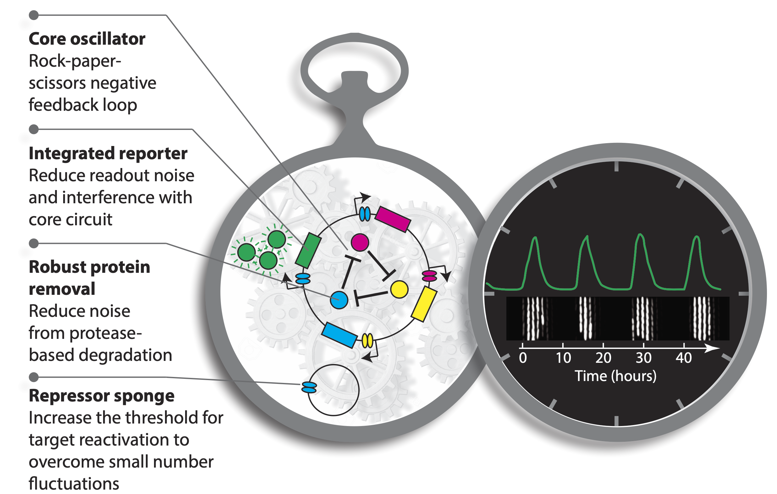
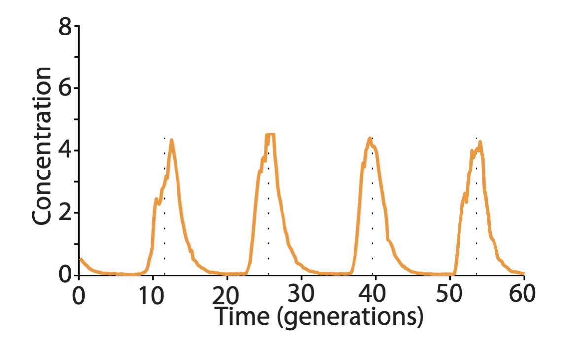
The long period repressilators were enabled in part by not destabilizing the proteins, making dilution through growth the only mechanism of protein removal. Despite their long periods, this circuit was incredibly precise. The standard deviation in period length was about 14%, and the pulse shape and amplitude was incredibly regular, as you can see in the image below.
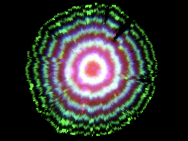
In fact, this circuit is so precise that even though cells are not synchronized with one another, they stay in sync over many generations of growth. When the cells grow as a colony on a plate, most growth occurs at the leading edge of the colony. Behind that front, cells stop growing, effectively leaving a record of the state of their repressilators at each point in time, somewhat like tree rings, as shown in this image:
One might have imagined that increasing the precision of the repressilator would require additional regulatory circuitry, but this does not seem to be the case, at least under these well-controlled conditions. As we wrote in an accompanying piece, “Evidently, precision does not necessarily demand circuit complexity and, in this case, even seems to benefit from minimalism.”. At the same time, achieving a constant period irrespective of growth conditions will likely require compensation mechanisms, much as early navigational clocks required additional systems to compensate for the effects of varying temperature on clock period.
Ring phases enable inference of bacterial growth dynamics
Last year, Pam Silver and colleagues took advantage of the incredible precision offered by this circuit to interrogate bacterial growth dynamics in the mammalian gut Riglar, et al., 2019. Their approach relied on the ability to read out repressilator phase from colony ring phases. More specifically, they found that the phase of the repressilator in the initial cell that seeded the colony controls the radial phasing of the rings in the colony. Cells that are plated at the peak of reporter fluorescence produce colonies with a high intensity “dot” at the center, whereas cells plated at the trough of the oscillations have rings shifted by 180 degrees. This is shown schematically in part c of the image below. They also took advantage of the ability to modulate the phase of the repressilator directly with two small molecule drugs, anhydrotetracycline (aTc) and IPTG, which respectively inhibit TetR and LacI proteins (a, below). After using these drugs to synchronize a population of cells at one phase, they could observe a beautiful linear relationship between the repressilator phase (as determined by the phasing of colony rings) and the elapsed growth of the cells (bottom-right plot, below). Further, they verified that it was really growth and not time per se that correlated with phase (see Figure 3 of the paper).
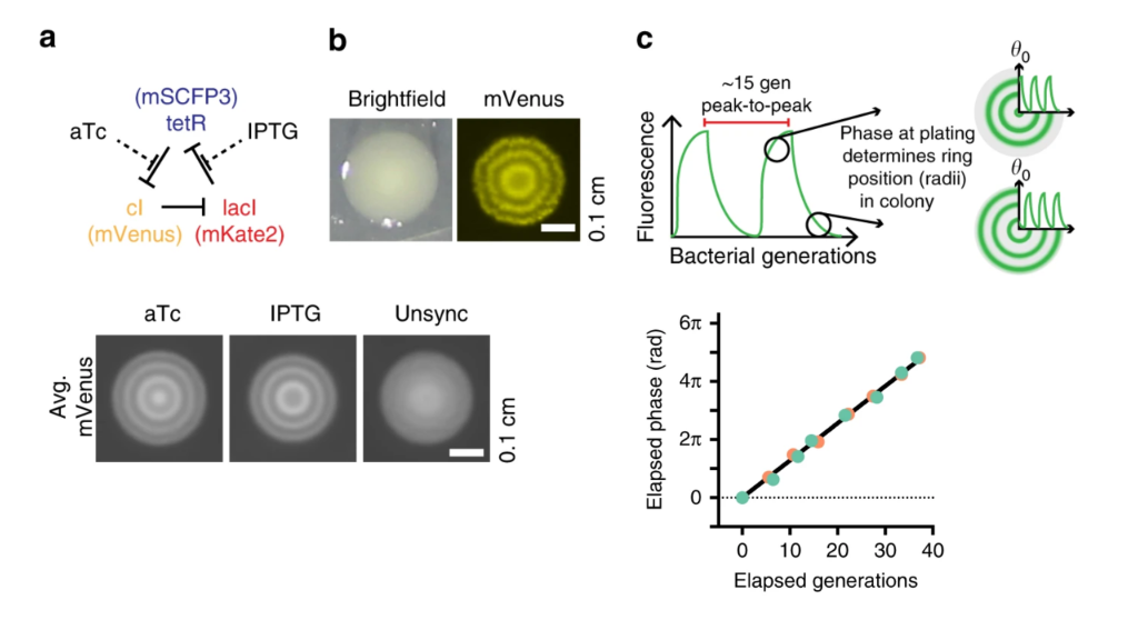
Colony phasing indicates cumulative cell growth. (a) The repressilator can be perturbed by adding the drugs aTc and IPTG, which inhibit TetR and LacI, respectively. This allows one to put the system into a defined phase. (b) Colony showing the rings of fluorescent protein expression that indicate phase. (c) Schematic indicating how repressilator phase correlates with colony ring phase. (lower left) Examples of colonies generated by cells exposed to either aTc or IPTG. Note the distinct phasing. (lower right) Colony ring phase correlates with number of generations of growth.
Taken together, this means that the phase of the oscillator can be used as a measure of bacterial growth. The repressilator has become a growth readout.
They wondered whether this might allow one to recover the history of cell growth in an environment that would otherwise be inaccessible. E. coli normally spend part of their life cycle in mammalian gut, but, as you can imagine, it’s hard to observe what’s going on there directly. If we could see what was going on, it would both provide insight into how much cells typically grow within the gut, how much cell-cell variability there is in that growth, and how the amount of growth depends on conditions in the gut, including which other bacteria are present, or whether it has been recently depleted of bacteria by antibiotics. In fact, with this approach, they identified conditions, such as inflammation, that led to greater variability in growth. They also saw that growth varied between different spatial areas or niches in the gut.
This work demonstrates a few key points:
Even a relatively simple synthetic circuit of three genes can operate with incredible precision in a living cell.
Synthetic circuits like the repressilator can provide unique functionality both to analyze biological systems (as in this example) and, increasingly, to provide useful new functions such as therapeutics. In this case, one could imagine further exploring how engineered probiotic cells behave when introduced into animals.
The three-repressor structure of the repressilator, and the way its dynamics progress sequentially from expression of one repressor to the next, means that one can define the phase of the oscillator. Phase is a critical aspect of many natural biological oscillators. For example, the cell cycle is controlled by an oscillator that advances a cell from one phase to the next, in a sequential cycle, with each phase performing unique activities. These phases begin with growth during G1 phase, followed by DNA replication during S phase, a second G phase (G2), and finally an M phase corresponding to mitosis.
Part II: Less is more, or the simplest oscillator
Next, we continue our discussion of oscillators by considering a very simple oscillator, even simpler than the repressilator, but based on a similar property of delayed negative feedback. Specifically, we consider a single-gene circuit with negative feedback with delay.
The basic idea has been put forward multiple times, notably by Julian Lewis in 2003, describing transcriptional delay.
Delayed negative feedback is actually quite familiar to anyone who has encountered a poorly designed hotel room thermostat. The thermostat will turn on the heater in response to cold temperatures, overheating the room beyond the set point before shutting off and letting it cool well below the target temperature before turning the heater back on. These types of overshoot dynamics are usually regarded as a problem to be eliminated by more sophisticated controller designs—-the major subject of control theory.
Let us consider a repressor that negatively autoregulates its own production, as in the diagram. The concentration of the protein does not instantaneously reflect the expression level of its own gene. For one thing, there are the transcription and translation steps we have already encountered. But there is also a second source of delay. The appearance of a freshly translated protein does not actually occur until translation is complete. That is, there is a delay between the initiation and completion of translation for each protein. (By contrast, translation can occur co-transcriptionally in bacteria, so translation does not have to wait to start before transcription is finished.)
In E. coli, translation occurs at a rate of about 15 amino acids per second. So a sizable protein like β-galactosidase can take more than a minute to translate.
In eukaryotic cells, where gene expression has additional steps, including splicing and nuclear export, these delays can be even longer. In fact, a totally different synthetic single gene negative autoregulation oscillator circuits was implemented in eukaryotic cells using the variability in intron length (Swinburne, et al., Genes and Dev., 2008), rather than translational delay per se, to delay protein production.
An example of delay in a biological circuit
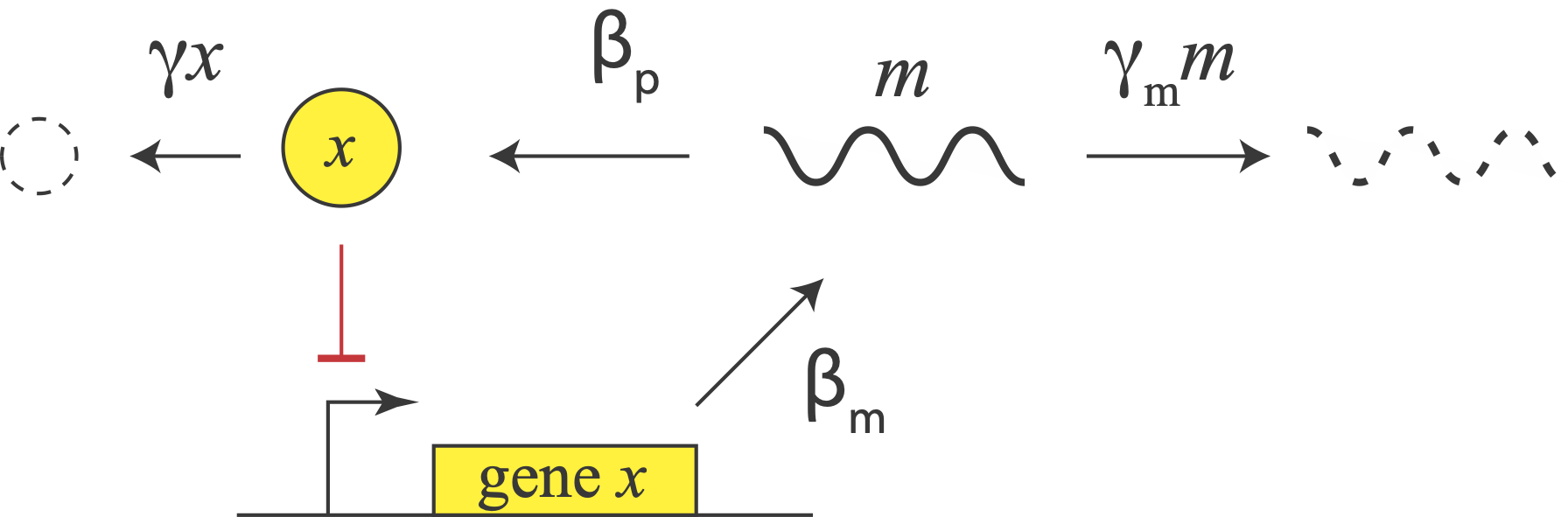
To investigate how molecular details can give rise to delay (which in turn can give oscillations), we consider a multistep process of the production and action of a repressor. The delay in transcriptional regulation in real cells comes from processes such as translation, trans-nuclear transport, etc. We will consider a simple version of this, shown below, in which \(r\) is some intermediate state en route to functioning protein.
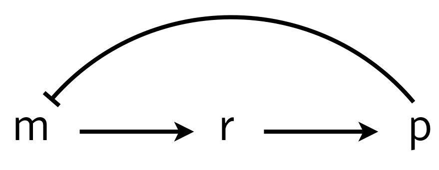
We can write the dynamics as
\begin{align} \frac{\mathrm{d}m}{\mathrm{d}t} &= \frac{\beta_{m}}{1 + (p/k)^n} - \gamma_m m,\\[1em] \frac{\mathrm{d}r}{\mathrm{d}t} &= \beta_{r} m - \gamma_r r,\\[1em] \frac{\mathrm{d}p}{\mathrm{d}t} &= \beta_{p} r - \gamma_{p} p, \end{align}
where for simplicity we have assumed mass action type kinetics for all processes other than repression. These equations can be nondimensionalized by renaming parameters and variables as \(r \leftarrow \gamma_m t\), \(p \leftarrow p/k\), \(m \leftarrow \beta_{r}\beta_{p} m/\gamma_m^2 k\), \(r \leftarrow \beta_{p} r/\gamma_m k\), \(\beta \leftarrow \beta_{m} \beta_{r} \beta_{p}/\gamma_m^2 k\) and \(\gamma \leftarrow \gamma_{p}/\gamma_m\) to give
\begin{align} \frac{\mathrm{d}m}{\mathrm{d}t} &= \frac{\beta}{1 + p^n} - m,\\ \frac{\mathrm{d}r}{\mathrm{d}t} &= m - r,\\ \frac{\mathrm{d}p}{\mathrm{d}t} &= r - \gamma p. \end{align}
There is a single fixed point \((m_0, r_0, p_0)\) for this system,
\begin{align} m_0 &= r_0 = \gamma p_0,\\ \frac{\beta}{\gamma} &= p_0(1+p_0^n). \end{align}
We can perform linear stability analysis about this fixed point, just as we did in for the repressilator.
\begin{align} \frac{\mathrm{d}}{\mathrm{d}t}\begin{pmatrix} \delta m \\ \delta r \\ \delta p \end{pmatrix} = \mathsf{A}\cdot\begin{pmatrix} \delta m \\ \delta r \\ \delta p \end{pmatrix}, \end{align}
with
\begin{align} \mathsf{A} = \begin{pmatrix} -1 & 0 & -a \\ 1 & -1 & 0 \\ 0 & 1 & -\gamma \end{pmatrix}, \end{align}
where
\begin{align} a = \frac{\beta n p_0^{n-1}}{(1+p_0^n)^2} = \frac{\gamma n p_0^n}{1+p_0^n}. \end{align}
To find the eigenvalues, we write the characteristic polynomial as
\begin{align} -(1+\lambda)^2(\gamma+\lambda) - a = -\lambda^3 - (2+\gamma)\lambda^2 - (1+2\gamma)\lambda -\gamma - a = 0. \end{align}
This polynomial has no positive real roots and either one or three negative real roots according to the Descartes Sign Rule. We are interested in the case where we have one negative real root and two complex conjugate roots. If the real part of these complex conjugate roots is positive, we have an oscillatory instability.
We can compute the eigenvalues of the linear stability matrix for various values of \(\beta\) and \(\gamma\) for fixed Hill coefficient \(n\). We will take a “brute force” approach and grid up \(\beta\)-\(\gamma\) space and compute the eigenvalues for each set of parameter values and determine if that point is stable or not. We can then display the linear stability diagram as an image, where a pixel is light colored in a stable region and dark colored in an unstable region.
[2]:
def fixed_point(beta, gamma, n):
    """Computes fixed point the m⟶r⟶p autorepression system.
    Uses np.roots because it has better convergence properties than
    scipy.optimize.fixed_point for integer n.
    """
    coeffs = np.zeros(n + 1)
    coeffs[0] = 1
    coeffs[-2] = 1
    coeffs[-1] = -beta / gamma
    p_0 = np.roots(coeffs)

    return p_0[(p_0.imag == 0) & (p_0 > 0)].real[0]


def lin_stab(beta, gamma, n):
    """Returns True if delay system is linearly stable and False
    otherwise.
    """
    p_0 = fixed_point(beta, gamma, n)

    # Linear stability matrix
    a = gamma * n * p_0 ** n / (1 + p_0 ** n)
    L = np.array([[-1, 0, -a], [1, -1, 0], [0, 1, -gamma]])

    # Compute eigenvalues
    lam = np.linalg.eigvals(L)

    return (lam.real < 0).all()


# Ultrasensitivity
n = 10

#
beta_vals = np.logspace(0, 4, 400)
gamma_vals = np.logspace(-1, 2, 400)

# Compute the linear stability diagram
stab = np.empty((len(beta_vals), len(gamma_vals)))
for i, beta in enumerate(beta_vals):
    for j, gamma in enumerate(gamma_vals):
        stab[i, j] = lin_stab(beta, gamma, n)

# Plot the result (shaded region has oscillatory instability)
p = bokeh.plotting.figure(
    plot_height=300,
    plot_width=350,
    x_axis_label="γ",
    y_axis_label="β",
    x_axis_type="log",
    y_axis_type="log",
    x_range=bokeh.models.Range1d(0.1, 100),
    y_range=bokeh.models.Range1d(1, 10000),
)
p.image([stab], x=0.1, y=1, dw=100, dh=10000, palette="Greys3", alpha=0.5)
p.text(x=0.45, y=100, text=["unstable"])
p.text(x=10, y=2, text=["stable"])

bokeh.io.show(p)
Importantly, we see that we must have very high ultrasensitivity (\(n\) about 9 or 10) to get oscillatory instabilities for reasonable values of \(\beta\) and \(\gamma\). Furthermore, the sliver of parameter space that gives an oscillatory instability is small. For such a simple mechanism for delay, the presence of oscillations are not robust to variations in parameter values and high sensitivity is necessary.
Differential equations with explicit delays
Above, we inserted extra biochemical steps into a process. But what if there is a real delay in a process, such as the delay betweeen initiation of translation and appearance of the fully synthesized and active protein? Or a delay between transcription initiation and nuclear export and translation initiation of the corresponding mRNA? To gain deeper insights on how delays affect stability, we will treat these situations with delay differential equations.
These days, we have an all too real example of delayed dynamics in the present COVID-19 pandemic. With this disease, the onset of symptoms occurs after a delay of many days from initial infection. Similarly, recovery or death also occur only many days after the symptoms appear. As a result, delay differential equations represent a useful framework for modeling the pandemic. Even more realistically, there is not a single fixed value for the delay in these cases but rather a distribution of different delays.
We will denote the time delay \(\tau\) and write down a delay differential equation, or DDE, describing the dynamics of expression of a gene, \(x\).
\begin{align} \frac{\mathrm{d}x}{\mathrm{d}t} = \frac{\beta}{\displaystyle{1+\left(\frac{x(t-\tau)}{k}\right)^n}} - \gamma x. \end{align}
This resembles are previous examples of negative autoregulation, except now the expression \(x(t-\tau)\) in the denominator on the right hand side of this equation indicates that the expression of \(x\) at time \(t\) depends on its expression level at an earlier time \(t - \tau\).
Doing our usual nondimensionalization, setting \(\beta \leftarrow \beta/\gamma\), \(t\leftarrow \gamma t\), \(x\leftarrow x/k\), and \(\tau \leftarrow\gamma \tau\), we have
\begin{align} \frac{\mathrm{d}x}{\mathrm{d}t} = \frac{\beta}{1+(x(t-\tau))^n} - x. \end{align}
We can solve this numerically to get oscillations, which we will do momentarily.
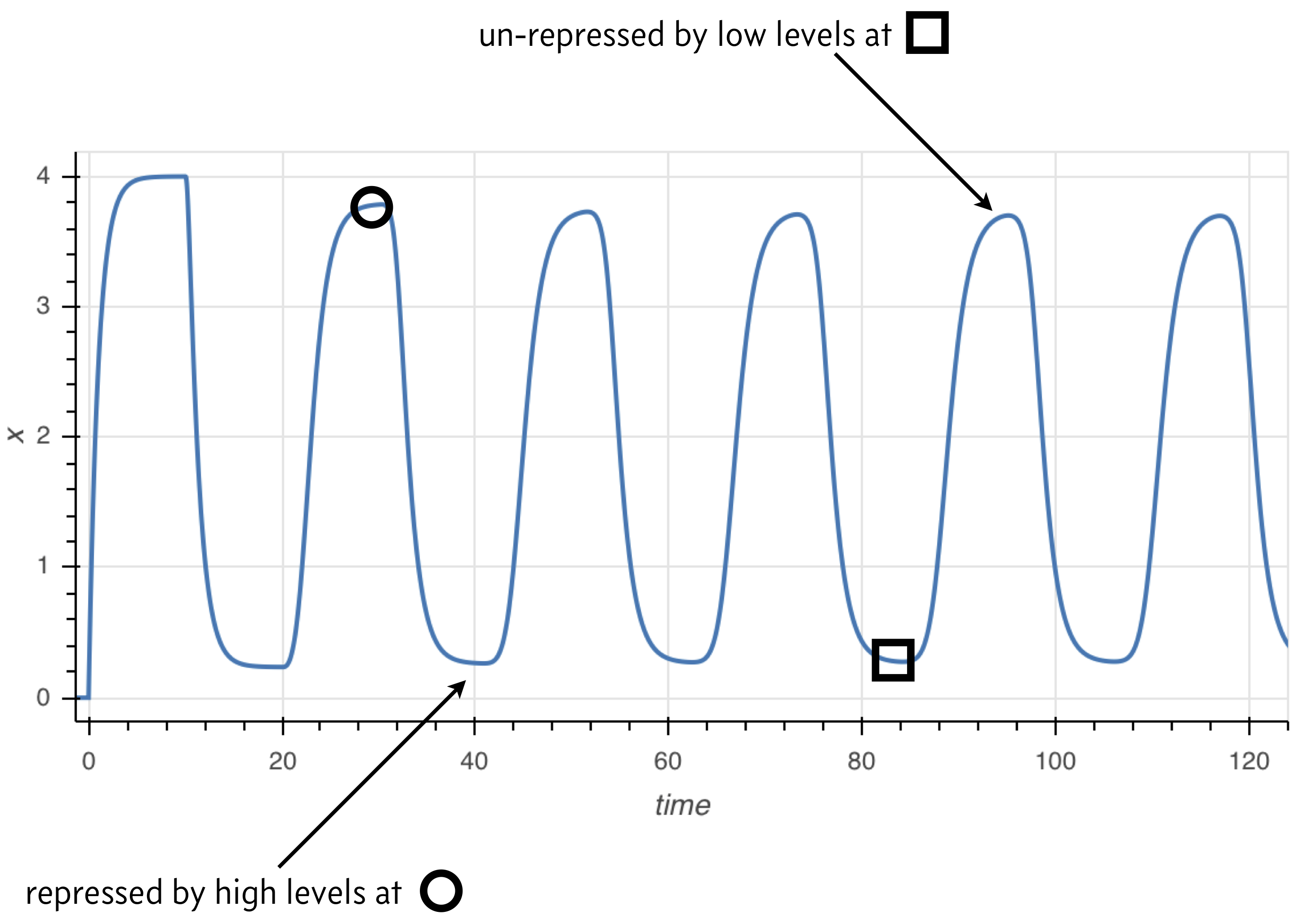
The principle behind the presence of oscillations is simple, and illustrated in the image below. Because the rate of expression is determined by past protein levels, high expression occurs when protein levels were low in the past and low expression occurs when protein levels were high in the past.
Numerical solution of DDEs
In general, we may write a system of DDEs as
\begin{align} \frac{\mathrm{d}\mathbf{u}}{\mathrm{d}t} = &= \mathbf{f}(t, \mathbf{u}(t), \mathbf{u}(t-\tau_1), \mathbf{u}(t-\tau_2), \ldots, \tau_n), \end{align}
where \(\tau_1, \tau_2, \ldots, \tau_n\) are the delays with \(\tau_1 < \tau_2 < \ldots < \tau_n\). We define the longest delay to be \(\tau_n = \tau\) for notational convenience. If we wish to have a solution for time \(t \ge t_0\), we need to specify initial conditions that go sufficiently far back in time,
\begin{align} y(t) = y_0(t) \text{ for }t_0-\tau < t \le t_0. \end{align}
The approach we will take is the method of steps. Given \(y_0(t)\), we integrate the differential equations from time \(t_0\) to time \(t_0 + \tau\). We store that solution and then use it to integrate again from time \(t_0+\tau\) to time \(t_0 + 2\tau\). We continue this process until we integrate over the desired time span.
Because we need to access \(y(t-\tau_i)\) at time \(t\), and \(t\) can be arbitrary, we often need an interpolation of the solution from the previous time steps. We will use SciPy’s functional interface for B-spline interpolation, using the scipy.interpolate.splrep() and scipy.interpolate.splev() functions.
We write the function below to solve DDEs with similar call signature as scipy.integrate.odeint().
ddeint(func, y0, t, tau, args=(), y0_args=(), n_time_points_per_step=200)
The input function has a different call signature than odeint() because it needs to allow for a function that computes the values of y in the past. So, the call signature of the function func giving the right hand side of the system of DDEs is
func(y, t, y_past, *args)
Furthermore, instead of passing in a single initial condition, we need to pass in a function that computes \(y_0(t)\), as defined for initial conditions that go back in time. The function has call signature
y0(t, *y0_args)
We also need to specify tau, the longest time delay in the system. Finally, in addition to the additional arguments to func and to y0, we specify how many time points we wish to use for each step to build our interpolants. Note that even though we specify tau in the arguments of ddeint(), we still need to explicitly pass all time delays as extra args to func. This is because we could in general have more than one delay, and only the longest is pertinent for the
integration.
[3]:
def ddeint(func, y0, t, tau, args=(), y0_args=(), n_time_points_per_step=200):
    """Integrate a system of delay differential equations.
    """
    t0 = t[0]
    y_dense = []
    t_dense = []

    # Past function for the first step
    y_past = lambda t: y0(t, *y0_args)

    # Integrate first step
    t_step = np.linspace(t0, t0 + tau, n_time_points_per_step)
    y = scipy.integrate.odeint(func, y_past(t0), t_step, args=(y_past,) + args)

    # Store result from integration
    y_dense.append(y[:-1, :])
    t_dense.append(t_step[:-1])

    # Get dimension of problem for convenience
    n = y.shape[1]

    # Integrate subsequent steps
    j = 1
    while t_step[-1] < t[-1] and j < 100:
        # Make B-spline
        tck = [scipy.interpolate.splrep(t_step, y[:, i]) for i in range(n)]

        # Interpolant of y from previous step
        y_past = lambda t: np.array(
            [scipy.interpolate.splev(t, tck[i]) for i in range(n)]
        )

        # Integrate this step
        t_step = np.linspace(
            t0 + j * tau, t0 + (j + 1) * tau, n_time_points_per_step
        )
        y = scipy.integrate.odeint(
            func, y[-1, :], t_step, args=(y_past,) + args
        )

        # Store the result
        y_dense.append(y[:-1, :])
        t_dense.append(t_step[:-1])

        j += 1

    # Concatenate results from steps
    y_dense = np.concatenate(y_dense)
    t_dense = np.concatenate(t_dense)

    # Interpolate solution for returning
    y_return = np.empty((len(t), n))
    for i in range(n):
        tck = scipy.interpolate.splrep(t_dense, y_dense[:, i])
        y_return[:, i] = scipy.interpolate.splev(t, tck)

    return y_return
Now that we have a function to solve DDEs, let’s solve the simple delay oscillator.
[4]:
# Right hand side of simple delay oscillator
def delay_rhs(x, t, x_past, beta, n, tau):
    return beta / (1 + x_past(t - tau) ** n) - x


# Initially, we just have no gene product
def x0(t):
    return 0


# Specify parameters (All dimensionless)
beta = 4
n = 2
tau = 10

# Time points we want
t = np.linspace(0, 200, 400)

# Perform the integration
x = ddeint(delay_rhs, x0, t, tau, args=(beta, n, tau))

# Plot the result
p = bokeh.plotting.figure(
    frame_width=450,
    frame_height=200,
    x_axis_label="time",
    y_axis_label="x",
    x_range=[t.min(), t.max()],
)
p.line(t, x[:, 0], line_width=2)

bokeh.io.show(p)
The ddeint() function is available as biocircuits.ddeint() package for future use.
Linear stability analysis of a delay differential equation
Consider a system of delay differential equations,
\begin{align} \frac{\mathrm{d}\mathbf{u}}{\mathrm{d}t} &= \mathbf{f}(\mathbf{u}(t), \mathbf{u}(t-\tau)). \end{align}
Here, we have written that the time derivative explicitly depends on the value of \(\mathbf{u}\) at the present time and also at some time \(\tau\) time units ago in the past. A steady state of the delay differential equations, \(\mathbf{u}_0\) satisfies \(\mathbf{u}_0(t) = \mathbf{u}_0(t-\tau) \equiv \mathbf{u}_0\) by the definition of a steady state. So, the steady state \(\mathbf{u}_0\) satisfies \(\mathbf{f}(\mathbf{u_0}, \mathbf{u}_0) = 0\). We will perform a linear stability analysis about this steady state.
To linearize, we have to remember that \(\mathbf{f}\) is a function of two sets of variables, present and past \(\mathbf{u}\). We write a Taylor series expansion with respect to both of these variables to linearize.
\begin{align} \mathbf{f}(\mathbf{u}(t), \mathbf{u}(t-\tau)) \approx \mathbf{f}(\mathbf{u}, \mathbf{u}_0) + \mathsf{A}\cdot(\mathbf{u}(t) - \mathbf{u}_0) + \mathsf{A}_{\tau}\cdot(\mathbf{u}(t-\tau) - \mathbf{u}_0), \end{align}
where
\begin{align} \mathsf{A} = \begin{pmatrix} \frac{\partial f_1}{\partial u_1(t)} & \frac{\partial f_1}{\partial u_2(t)} & \cdots \\[0.5em] \frac{\partial f_2}{\partial u_1(t)} & \frac{\partial f_2}{\partial u_2(t)} & \cdots \\ \vdots & \vdots & \ddots \end{pmatrix} \end{align}
and
\begin{align} \mathsf{A}_{\tau} = \begin{pmatrix} \frac{\partial f_1}{\partial u_1(t-\tau)} & \frac{\partial f_1}{\partial u_2(t-\tau)} & \cdots \\[0.5em] \frac{\partial f_2}{\partial u_1(t-\tau)} & \frac{\partial f_2}{\partial u_2(t-\tau)} & \cdots \\ \vdots & \vdots & \ddots \end{pmatrix}, \end{align}
where all derivatives in both matrices are evaluated at \(\mathbf{u}(t) = \mathbf{u}(t-\tau) = \mathbf{u}_0\). Defining \(\delta\mathbf{u} = \mathbf{u} - \mathbf{u}_0\), our linearized differential equations are
\begin{align} \frac{\mathrm{d}\delta\mathbf{u}}{\mathrm{d}t} = (\mathsf{A} + \mathsf{A}_{\tau})\cdot \delta\mathbf{u}. \end{align}
To solve the linear system, we insert the ansatz, \(\delta\mathbf{u} = \mathbf{w}\,\mathrm{e}^{\lambda t}\), giving
\begin{align} \lambda \mathrm{e}^{\lambda t}\,\mathbf{w} = \mathsf{A}\cdot\mathbf{w}\,\mathrm{e}^{\lambda t} + \mathsf{A}_{\tau}\cdot \mathbf{w}\,\mathrm{e}^{\lambda (t-\tau)}, \end{align}
or, upon simplifying,
\begin{align} \lambda \mathbf{w} = (\mathsf{A} + \mathrm{e}^{-\lambda \tau} \mathsf{A}_{\tau})\cdot \mathbf{w}. \end{align}
So, \(\lambda\) is an eigenvalue and \(\mathbf{w}\) is the corresponding eigenvector for the matrix \((\mathsf{A} + \mathrm{e}^{-\lambda \tau} \mathsf{A}_{\tau})\). In general, there are infinitely many values of \(\lambda\). Nonetheless, if we can show that the real part of all possible values of \(\lambda\) is less than zero, then the fixed point is stable. Otherwise, if the real part of any values of \(\lambda\) are positive, the fixed point is locally unstable. If \(\lambda\) has an imaginary part for the eigenvalues with a positive real part, the instability is oscillatory.
Linear stability analysis of delayed autorepression
We consider now the simple case of an autorepressor with delay.
\begin{align} \frac{\mathrm{d}x(t)}{\mathrm{d}t} = \frac{\beta}{1 + (x(t-\tau))^n} - x(t). \end{align}
The steady state \(x_0\) is given by setting the time derivative to zero,
\begin{align} \beta = x_0(1+x_0^n). \end{align}
The \(x_0\) that satisfies this equality is unique because the right hand is monotonically increasing from zero, so it only crosses a value of \(\beta\) once. So, we will consider the stability of this unique steady state.
We linearize the right hand side of the ODE around the fixed point. The matrices \(\mathsf{A}\) and \(\mathsf{A}_{\tau}\) are scalars in this case because we have a single species. Remember that the eigenvalue of a scalar is just the scalar itself. So, we have
\begin{align} &\mathsf{A} = -1 \\[1em] &\mathsf{A}_{\tau} = -\frac{\beta n x_0^{n-1}}{(1+x_0^n)^2} = -\frac{nx_0^n}{1+x_0^n} \equiv -a_{\tau}, \end{align}
where we have defined \(a_{\tau}\) (which must be positive) for convenience. Thus, our characteristic equation is
\begin{align} \lambda = -1 - a_{\tau}\mathrm{e}^{-\lambda \tau}. \end{align}
There are infinitely many \(\lambda\) that satisfy this equation in general. Nonetheless, we can still make progress. We write \(\lambda = a + ib\), where \(a\) is the real part at \(b\) is the imaginary part. Then, the characteristic equation is
\begin{align} a + ib = -a_{\tau} \mathrm{e}^{-a\tau} \mathrm{e}^{-ib\tau} - 1 = -a_{\tau}\mathrm{e}^{-a\tau}(\cos b\tau - i\sin b\tau) - 1. \end{align}
This can be written as two equations by equating the real and imaginary parts of both sides of the equality.
\begin{align} a &= -(1+a_{\tau} \mathrm{e}^{-a\tau} \cos b\tau ) \\[1em] b &= a_{\tau} \mathrm{e}^{-a\tau} \sin b\tau. \end{align}
Right away, we can see that if \(a\) is positive, we must have \(a_{\tau} > 1\), since \(\left|\mathrm{e}^{-a\tau}\cos b\tau\right| < 1\). Recall our expression for \(a_{\tau}\),
\begin{align} a_{\tau} = \frac{nx_0^n}{1+x_0^n}. \end{align}
Because \(x_0^n/(1+x_0^n) < 1\), we must have \(n>1\) in order to have the eigenvalue have a positive real part and therefore have an instability. So, ultrasensitivity is a requirement for a simple delay oscillator.
To investigate when we get an oscillatory instability, we will compute the values of \(a_{\tau}\) and \(\tau\) that lie on the bifurcation line between a stable steady state and an oscillatory instability, a so-called Hopf bifurcation. To do this, we solve for the line with \(a = 0\) and \(b \ne 0\). In this case, the characteristic equation gives
\begin{align} -a_{\tau} \cos bt &= 1 \\[1em] a_{\tau} \sin bt &= b. \end{align}
Squaring both equations and adding gives
\begin{align} a_{\tau}^2 = 1 + b^2, \end{align}
Thus,
\begin{align} b = \sqrt{a_{\tau}^2 - 1}, \end{align}
which can only hold for \(a_{\tau} > 1\), which we already found was a requirement for an oscillatory instability. To find \(\tau\), we have
\begin{align} &-a_{\tau} \cos b\tau = -a_{\tau} \cos \sqrt{a_{\tau}^2 - 1}\,t = 1 \\[1em] &\Rightarrow\; \tau = \frac{\pi - \cos^{-1}\left(a_{\tau}^{-1}\right)}{\sqrt{a_{\tau}^2 - 1}}. \end{align}
The region of stability is below the bifurcation line in the \(\tau\)-\(\beta\) plane, since a smaller \(\tau\) serves to decrease the real part of \(\lambda\).
Now that we have worked it out analytically, we can compute and plot the linear stability diagram in the \(\tau\)-\(\beta\) plane.
[5]:
def fp_rhs(x, beta, n):
    return beta / (1 + x ** n)


def bifurcation_line(beta, n):
    x_0 = scipy.optimize.fixed_point(fp_rhs, 1, args=(beta, n))
    a_tau = n * x_0 ** n / (1 + x_0 ** n)

    if a_tau <= 1:
        return np.nan

    return np.arccos(-1 / a_tau) / np.sqrt(a_tau ** 2 - 1)


# Set up values for plotting
n_vals = (1.2, 2, 5, 10)
beta = np.logspace(-0.2, 2, 2000)

# Set up plot
p = bokeh.plotting.figure(
    frame_width=300,
    frame_height=300,
    x_axis_label="β",
    y_axis_label="τ",
    x_axis_type="log",
    y_axis_type="log",
    x_range=[0.8, 100],
    y_range=[0.1, 25],
)

# Compute bifurcation lines and plot
colors = bokeh.palettes.Blues8[::-1]
for i, n in enumerate(n_vals):
    tau = np.array([bifurcation_line(b, n) for b in beta])
    p.patch(
        np.append(beta, beta[-1]),
        np.append(tau, np.nanmax(tau)),
        color="gray",
        alpha=0.2,
        level="underlay",
    )
    p.line(beta, tau, color=colors[i + 2], legend_label=f"n={n}", line_width=2)
p.text(x=10, y=1, text=["unstable"])
p.text(x=1, y=0.2, text=["stable"])

bokeh.io.show(p)
Note that for longer delays, provided the promoter is not too weak (\(\beta > 1\)), the region for which there is an oscillatory instability is very large. Thus, in the large \(\tau\) regime, the presence of oscillations is robust to changes in other parameter values.
Synthetic single gene oscillators oscillate
Can a single gene oscillator actually oscillate? In fact, it can! Stricker et built a simple negative autoregulatory circuit, in which the LacI repressor represses its own expression as well as the expression of a fluorescent protein, as in the following diagram:
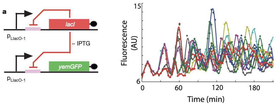
Then, they analyzed the dynamics of this circuit in bacteria that were grown in a microfluidic device to keep them under relatively constant environmental conditions. During growth, they recorded movies and tracked individual cells. The oscillations of individual cells are apparent in the plot to the right, as they are in the movie below.
Part III: Positive-negative feedback loops decouple period and amplitude
We have now explored several ways that delayed negative feedback can generate oscillations and how those oscillations may be useful. You may be thinking all there is to oscillators is delayed negative feedback. In fact, a distinct positive-negative feedback architecture occurs naturally and has been constructed and analyzed synthetically. In these systems, an activator stimulates its own expression and that of a repressor. The repressor, in turn, represses the activator and itself. Thus, this topology comprises three feedback loops involving two proteins.
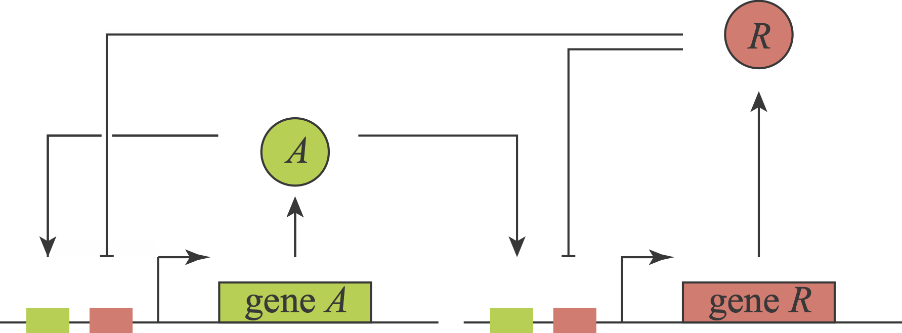
What an amazing circuit! Gaze at it and appreciate how it combines features of so many of the systems we have now encountered. Its positive autoregulatory “A” feedback loop could, with ultrasensitivity, produce bistability. Its negative autoregulation module could, with a delay and ultrasensitivity, generate oscillations. Further, these two loops are intertwined with one another in an intriguing way, each regulating the other. Finally, notice that in this circuit, as with the feed-forward loops, we encounter combinatorial regulation: each of the two genes is co-regulated by two distinct inputs, A and R. Here, the combinatorial regulation is similar for both genes (A activates and R represses). These combinatorial inputs could combine in an AND-like, OR-like or some other fashion.
The behavior of this type of circuit was by Hasty et al (PRL, 2002). We will analyze it in greater detail in a homework problem. Circuits like this can act as “relaxation oscillators.” In this regime, a complete oscillation occurs in 4 phases:
A flips itself on through the positive feedback loop.
R builds up slowly.
Once R reaches a sufficiently high concentration, it inhibits A’s ability to keep itself on. As a result, A rapidly shuts off.
With A no longer present, R synthesis stops and existing R slowly decays. When R is low enough for A to flip itself back on, repeating the cycle. This cycle is favored under certain conditions. A should be bistable and have faster kinetics (faster degradation rates) than R. At the promoters, the ability of R to repress must dominate the ability of A to activate.
Tsai, Ferrell, and coworkers pointed out (Science, 2008) that regulatory architectures like this—whether implemented through gene regulation or at other levels—are remarkably prevalent across diverse biological oscillators, as shown in this table from their paper:
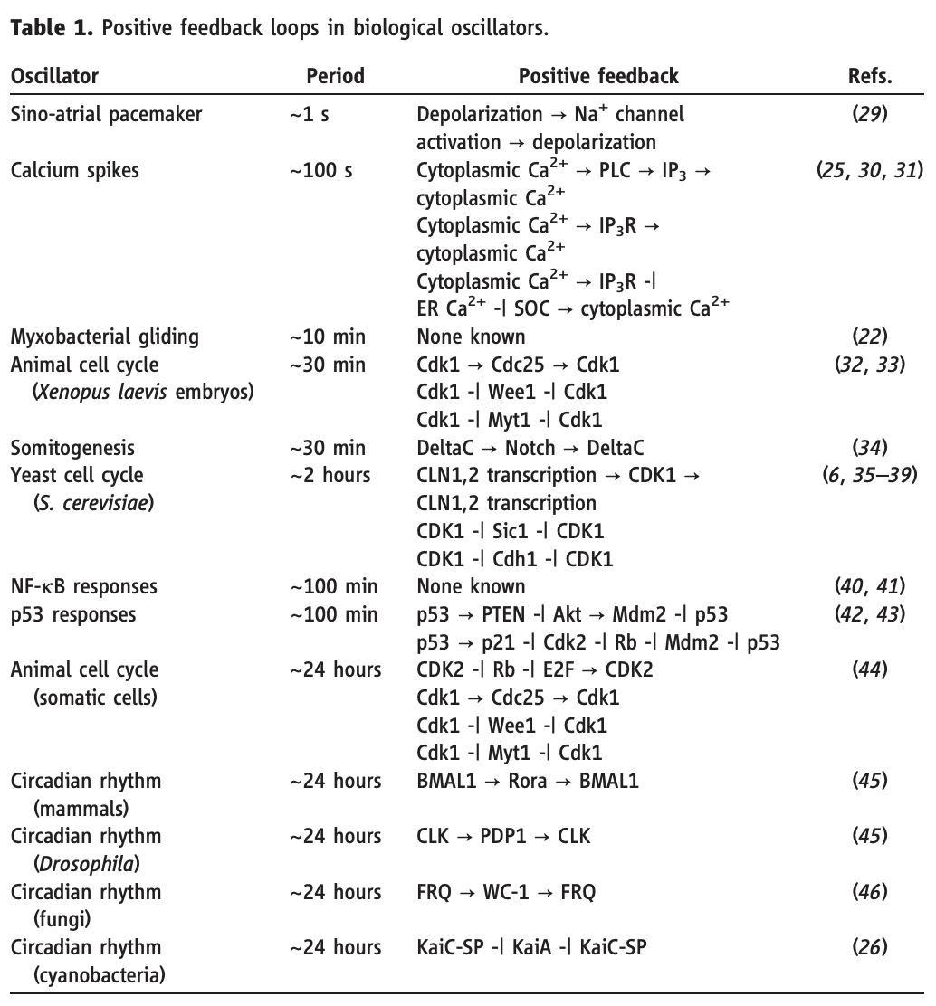
They further suggested an intriguing reason: The positive-negative architecture decouples two key features of the oscillator: its amplitude, which is set by the bistable positive feedback loop of A, and its period, which is determined by the slow decay rate of R. Decoupling these two features enables biological systems to independently tune them. For example, in the sino-atrial node, which functions as the natural pacemaker for the heart, the frequency of heartbeats is regulated independently of their amplitude. Similarly, they suggested, the period of the cell cycle may need to be regulated independently without altering the peak concentrations of the activated cyclin-dependent kinases that it controls.
In contrast to the positive-negative oscillators, in pure negative feedback oscillators, most parameters tend to tune period and amplitude together. For example, in the repressilator, increasing the gene expression strength \(\beta\) increases the peak concentrations of each protein. But this in turn means that it takes correspondingly longer for each repressor to decay low enough to relieve its repression. As a result, one gets a longer period as well as a higher amplitude. Similar results hold for other parameter variations.
Experimental realization of the positive-negative oscillator:
In 2008, Hasty’s lab described a synthetic implementation of the positive-negative oscillator (Nature, 2008). As a repressor, they used LacI, as in the repressilator. As an activator, they repurposed AraC, a well-characterized transcriptional activator whose normal role is to control arabinose utilization genes in E. coli. They also incorporated a fluorescent reporter gene to interrogate what was happening.
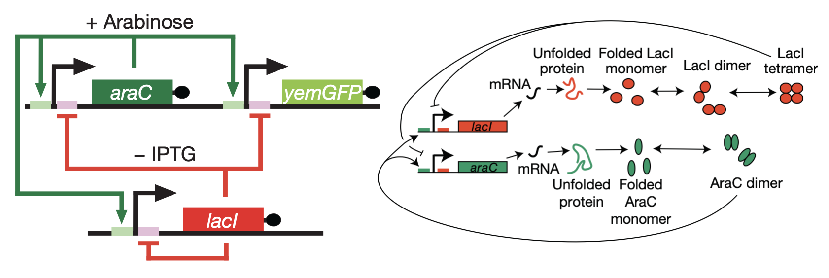
Using this design, they obtained beautiful oscillations, seen in the movie below, and further showed tunability of the oscillator.
Conclusions
To conclude, we have now explored several principles of oscillator design and an example of its application. To summarize the previous lecture along with this one, we see:
Delayed negative feedback can generate self-sustaining limit cycle oscillations.
The repressilator design implements delayed negative feedback through a three component rock-scissors-paper architecture.
Linear stability analysis reveals that the repressilator design can oscillate for large enough promoter strengths and high enough ultrasensitivity. Oscillations are also facilitated by low leakiness and similar mRNA and protein decay rates.
The repressilator can be made to operate with extremely high precision, with a few simplifications.
This property enables its use as a cell autonomous growth probe in mammalian gut.
Even simpler single-component oscillator designs are also possible, although their ability to oscillate can be more sensitive to parameters.
These systems can be treated using delay differential equations, in which the rate of change of a component now depends on the concentrations of system components some time ago.
Finally, combining negative and positive feedback loops enables relaxation oscillators. These exist in many natural systems, and offer a key benefit: the ability to independently tune amplitude and period.
Computing environment
[6]:
%load_ext watermark
%watermark -v -p numpy,scipy,bokeh,jupyterlab
CPython 3.7.7
IPython 7.13.0

numpy 1.18.1
scipy 1.4.1
bokeh 2.0.1
jupyterlab 1.2.6