14. Cellular ‘bet-hedging’
Design principle
When environmental conditions fluctuate unpredictably, bet-hedging through spontaneous, probabilistic cellular state-switching (differentiation) can outperform adaptive response strategies.
Concepts
Optimal (Kelly) betting
Antibiotic persistence
Biological bet-hedging
Techniques
Optimal betting strategies
Single cell movies
[1]:
import numpy as np

import biocircuits

import bokeh.io
import bokeh.plotting

bokeh.io.output_notebook()
Survival in an uncertain world requires adaptability and anticipation, the complementary abilities to respond to and prepare for change.
— Jeffrey N. Carey and Mark Goulian, “A bacterial signaling system regulates noise to enable bet hedging,” Current Genetics, 2019.
Cellular investors
Consider a very loose analogy between bacteria and investing. If you have a crystal ball that can tell you the future, as well as some spare cash, then you could invest all of that cash in a single stock, the one you know will perform best over the period you care about. The difficulty of this strategy is that, even if you have the cash, you probably do not have the crystal ball. You do not know which stocks will take off, which will show some lackluster growth, and which will collapse entirely. Indeed, the value of any stock may depend not only on the underlying strength of the company but also on all sorts of unpredictable developments ranging from interest rates to pandemics. Confronted by this uncertainty, a common strategy is to spread one’s money across across multiple investments. One hopes that the strong performers will more than compensate for the weaker ones. And if any individual stock fails, one would not lose everything. This is a form of bet hedging.
Bacteria face a similar challenge. Individual cells can exist in a variety of physiological states, each of which may be adapted to some but not all potential future environments. A bacterial cell that anticipates the environment it will soon face can proliferate more rapidly than its cousins. By contrast, in the wrong state and it may grow more slowly or not survive the coming environmental change at all.
Bacteria have evolved for billions of years anticipate future conditions. Nevertheless, just as future stock prices are hard to predict even for an expert investor, so too are environmental fluctuations in temperature, salt, toxins, antibiotics, and attacking immune cells all difficult or impossible to predict with certainty for our little bacterium. One can think of this is as a form of biological bet hedging in which the shared genome a clonal cell population spreads its bets, in the form of individual cells, across multiple physiological states, each adapted to different possible future environmental conditions.
The ideal cell for an uncertain world
Today, we seek to gain some insight into how bacteria can and do “bet.” We will imagine that we are designing a bacterial stress response system for a custom bacterium. Our goal is to maximize the survival and proliferation of our designer bug. We can provide the cell with an array of sensors, information processing circuits, and responses.
We also have the option, if we want, to incorporate a “random number generator” that operates independently in each individual cell. The random number generator is essential to allow these genetically identical cells to do different things in the same environment. And we have already seen how the cell generate randomness–through molecular noise! More specifically, we learned that gene expression occurs through intrinsically stochastic bursts of protein production. We further saw, through the example of bacterial competence, that this noise, when considered in the context of a regulatory circuit, enables cells to implement probabilistic strategies, by controlling the fraction of cells in the population that are in one state or another. The probabilities with which cells do one thing or another can, in general, depend on the environment, or even on its history.
Overview of this lecture:
First, because this is fundamentally a gambling, or betting, question, we will begin with some classic results in the theory of proportional gambling, or “Kelly betting,” described by John Kelly in 1956. We will follow an excellent and highly recommended lecture from Thomas Ferguson at UCLA.
Next, to see how to optimize growth bacterial growth, we will consider a minimal biological example based on stochastic switching between two cellular states and two environments.
We will then extend this discussion to systems with multiple states and multiple corresponding environments, to see if and when a purely probabilistic strategy can outperform one based on direct sensing of the environment.
Finally, we will highlight the particular phenomenon of antibiotic persistence, which presents a biomedical important example in which bacterial bet-hedging plays out.
A simple betting game
Following Ferguson, we start with the simplest betting game one can imagine: Each day you get to make a bet, and the odds of winning are always the same. Even better, unlike Vegas, the odds are actually in your favor, with your probability of winning, \(p\) , better than even: \(p>0.5\) .
All you have to decide is how much you want to bet each day. \(b_k\) denotes the amount of your \(k\)th bet. It could range from 0 to your total fortune before the bet, denoted \(X_{k-1}\). That is \(0\le b_k \le X_{k-1}\).
If you win or lose the bet, you gain or lose \(b_k\) dollars, respectively.
\begin{align} X_k = \begin{cases} X_{k-1} + b_k & \textrm{ with probability } p \\[1em] X_{k-1} - b_k & \textrm{ with probability } 1-p \end{cases} \end{align}
“I’m ruined!”
How much should you bet each day?
Each day, because \(p>1\), the bet that will maximize the “expectation value” of your wealth would be to bet everything, \(b_k=X_{k-1}\).
If you won every single bet, your wealth would increase, after \(k\) bets by a factor of \(2^k\). However, the probability of winning \(k\) bets in a row, \(p^k\), is low even when \(p\) is high. For instance, with \(p=0.8\), you have less than only about 1.5% chance of surviving 20 rounds. This is the phenomenon of gambler’s ruin.
Proportional betting
Since the odds are in your favor here, there ought to be a better strategy.
One possibility is proportional betting. In this scheme, you set the size of your bet to be proportional to the amount of money you have: \(b_k = f X_{k-1}\), where \(0<f<1\) denotes the fraction of your wealth you bet on each round. Even if you lose, you are not wiped out completely. You still live to play another day.
What is the best value of \(f\) to use in this scheme? Ideally, you would choose the value that maximizes the rate of increase of your wealth. That way, you can reach your own personal comfort level as fast as possible and find something more meaningful to do with your time.
Let’s consider one particular “run” of \(n\) bets, in which you won \(Z_n\) times and lost \(n-Z_n\) times. After this run, your wealth has now changed from \(X_0\) to
\begin{align} X_n = X_0 (1+f)^{Z_n}(1-f)^{n-Z_n}. \end{align}
Of course, each run will be different depending on \(Z_n\) and the distribution of possible \(Z_n\)’s is Binomial; \(Z_n \sim \text{Binom}(n,p)\). We can express expected fold change in wealth.
\begin{align} \frac{\langle Z_n\rangle}{Z_0} = \langle (1+f)^{Z_n}(1-f)^{n-Z_n}\rangle, \end{align}
which is in general difficult to calculate analytically. (We will do so by sampling out of the distribution of \(Z_n\) momentarily.) We can, however, compute the expected logarithm of the fold change in wealth.
\begin{align} \left\langle \ln \frac{Z_n }{Z_0}\right \rangle &= \left\langle Z_n \ln (1+f) + (n - Z_n)\ln (1-f) \right\rangle \\[1em] &= n\ln (1-f) + \langle Z_n \rangle \, [\ln (1+f) - \ln (1-f)] \\[1em] &= n\left[p \ln (1+f) + (1-p) \ln (1-f)\right], \end{align}
where in the last line we have used the fact that \(Z_n\) is Binomially distributed, so \(\langle Z_n \rangle = np\). We thus expect an exponential growth in wealth,
\begin{align} \mathrm{e}^{\langle \ln X_n\rangle} = X_0\,\mathrm{e}^{r n}, \end{align}
where the growth rate is
\begin{align} r = p \ln (1+f) + (1-p) \ln (1-f). \end{align}
This expression may remind you of Shannon’s information—in fact, Kelly’s 1956 article explores this connection and extends this analysis to many other interesting examples and connections.
Now we can answer the critical question: what is the optimal bet, \(f\)? To do so, just solve \(\frac{\mathrm{d}r}{\mathrm{d} f}=0\) to find the \(f\) that maximizes the growth rate. The result is
\begin{align} f_{opt} = \begin{cases} 2p - 1 & p > 1/2,\\[1em] 0 & p \le 1/2. \end{cases} \end{align}
[2]:
p = np.arange(0, 1, 0.05)
fopt = 2 * p - 1
fopt[np.where(fopt < 0)] = 0

pl = bokeh.plotting.figure(
    frame_width=350, frame_height=250, x_axis_label="p", y_axis_label="f_opt",
)

pl.line(p, fopt, line_width=2)

bokeh.io.show(pl)
For example, with a modest advantage like \(p=0.55\), you would bet 10% each time. With a larger advantage like \(p=0.9\), you could bet 80%.
A few interesting points about this result:
What if the odds are unfavorable? If \(p<1/2\), you are better off (of course) not betting.
This rule can be interpreted as maximizing the expectation value for the logarithm of total wealth.
This result can be generalized to the case where the probabilities change with time. In that case, each round one just replaces \(p\) with \(p_k\).
In his conclusion, Kelly writes:
The gambler introduced here follows an essentially different criterion from the classical gambler. At every bet he maximizes the expected value of the logarithm of his capital. The reason has nothing to do with the value function which he attached to his money, but merely with the fact that it is the logarithm which is additive in repeated bets and to which the law of large numbers applies. Suppose the situation were different; for example, suppose the gambler’s wife allowed him to bet one dollar each week but not to reinvest his winnings. He should then maximize his expectation (expected value of capital) on each bet. He would bet all his available capital (one dollar) on the event yielding the highest expectation. With probability one he would get ahead of anyone dividing his money differently.
See Tom Ferguson’s lecture for other interesting extensions and applications.
Simulating Kelly betting
We worked out the expectation value of the logarithm of wealth. We might also be interested in learning about how individual outcomes of Kelly betting might play out and to gather information about the distribution of outcomes. To that end, we can simulate Kelly betting games. We do so below, starting with \(X_0 = 1\) and betting 100 rounds, with \(p = 0.6\), giving an optimal betting strategy of \(f = 2p-1 = 0.2\).
[3]:
def kelly_bet(X, p, f):
    """Make a single bet using a Kelly strategy."""
    if np.random.random() < p:
        return X * (1 + f)
    else:
        return X * (1 - f)


def kelly_bet_series(X0, p, f, n_rounds):
    """Perform a series of Kelly bets."""
    X = np.empty(n_rounds + 1)
    X[0] = X0
    for i in range(n_rounds):
        X[i + 1] = kelly_bet(X[i], p, f)

    return X


# Kelly bets with 1 initial wealth points
X0 = 1
p = 0.6
f = 0.2
fbad1 = 0.1
fbad2 = 0.35

n_rounds = 100
n = np.arange(n_rounds + 1)

# Perform 10000 betting series
bets = np.array([kelly_bet_series(X0, p, f, n_rounds) for _ in range(10000)])
betsbad1 = np.array(
    [kelly_bet_series(X0, p, fbad1, n_rounds) for _ in range(10000)]
)
betsbad2 = np.array(
    [kelly_bet_series(X0, p, fbad2, n_rounds) for _ in range(10000)]
)

# Theoretical growth rate
r = p * np.log(1 + f) + (1 - p) * np.log(1 - f)

# Plot 100 betting series overlaid with expectations
pl = bokeh.plotting.figure(
    width=550,
    height=400,
    y_axis_type="log",
    x_axis_label="n",
    y_axis_label="riches",
)
for i in range(100):
    pl.line(n, kelly_bet_series(X0, p, f, n_rounds), alpha=0.2)

pl.circle(n, np.mean(bets, axis=0), color="orange", legend_label="〈Xn〉")
pl.circle(
    n,
    np.exp(np.mean(np.log(bets), axis=0)),
    color="purple",
    legend_label="exp(〈ln Xn〉)",
)
pl.line(
    n,
    X0 * np.exp(r * n),
    line_width=2,
    color="tomato",
    legend_label="X0 exp(rn)",
)
pl.legend.location = "top_left"

pl.line(
    n,
    np.exp(np.mean(np.log(betsbad1), axis=0)),
    color="green",
    line_width=1,
    legend_label="f=0.1: exp(〈ln Xn〉)",
)
pl.line(
    n,
    np.exp(np.mean(np.log(betsbad2), axis=0)),
    color="black",
    line_width=1,
    legend_label="f=0.3: exp(〈ln Xn〉)",
)


bokeh.io.show(pl)
Each series of bets is shown in a blue line, with the computed and theoretical expectation values shown. On average, the wealth grows, but we do occasionally lose. The green and black lines show suboptimal bets that are either too high or too low – with suboptimal results. You can play with this code to convince yourself that the optimal bet follows the analytical result.
It is also interesting to look at the distribution of outcomes: What is the distribution of outcomes after 100 rounds of betting? We can look at the ECDF of the betting outcomes.
[4]:
# Plot the ECDF (thinned, to limit the glyphs)
pl = biocircuits.ecdf(
    bets[::10, -1],
    x_axis_type="log",
    x_axis_label="riches",
    line_width=2,
    formal=True,
)
bokeh.io.show(pl)
We lose about 12% of the time, but we can still win big (the riches axis is on a logarithmic scale)!
What does this calculation have to do with bacteria? The key point here is that even when outcomes are unpredictable, there can be optimal betting strategies. Over billions of years, evolution may have found those strategies.
Alternative bacterial strategies: sense and respond or stochastically switch?
Here we ask how a population of cells can survive and even thrive in unpredictable environments. Just as we ask how we can grow our financial portfolio and avoid ruin, so too we can ask how a clonal population of cells, implementing identical, but probabilistic, programs, can maximize their total growth rate and avoid elimination.
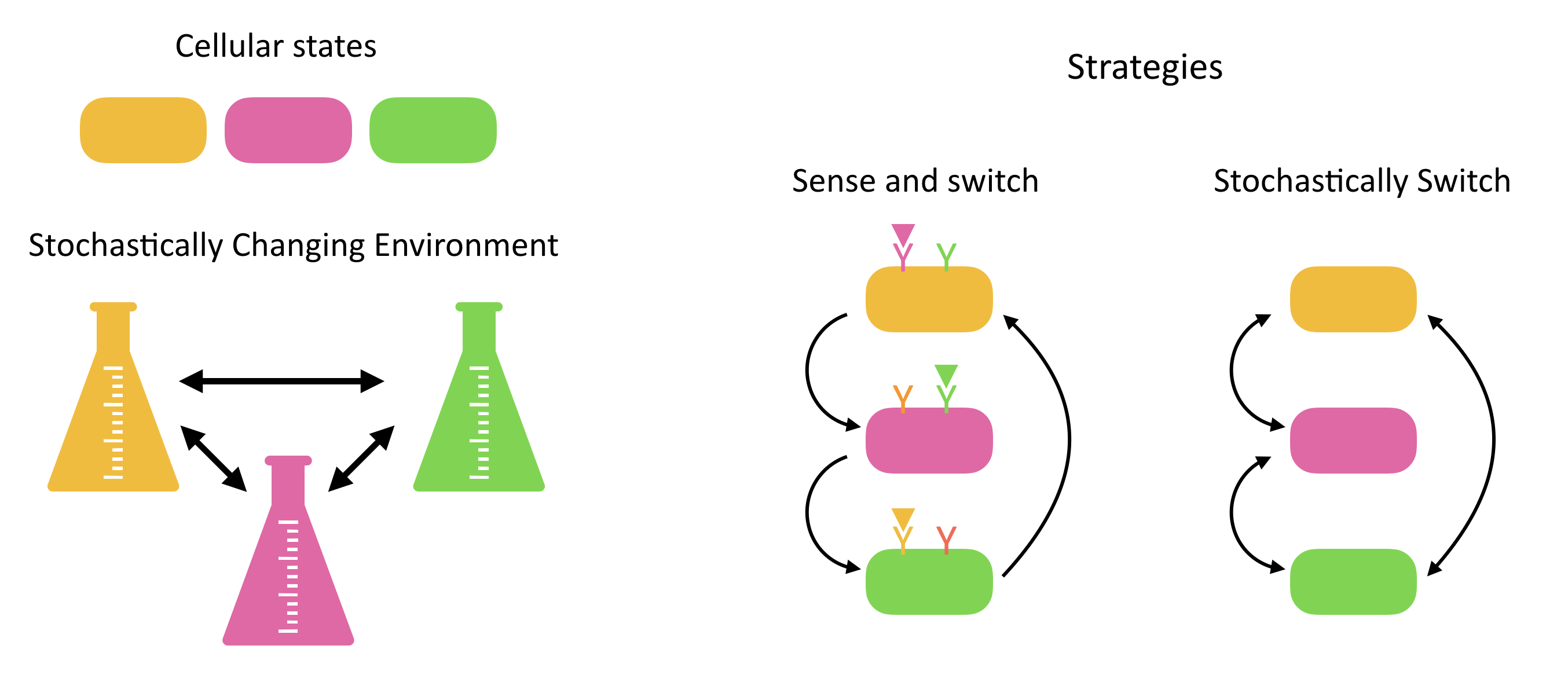
Responsive switching. At first glance, the most straightforward solution is to deterministically sense the current and environment and adjust expression of proteins to put cells into its best adapted state. However, this requires that cells express specific sensors for a broad variety of conditions that they may not encounter most of the time.
Stochastic switching. An alternative way to adapt is not to sense at all, but rather to just switch stochastically between different states, “hoping” that the cost from having cells in less adaptive states some of the time will be outweighed by the reduced cost of constantly sensing a broad variety of different inputs. In fact, many natural systems appear to implement such stochastic state-switching strategies.
Of course, both strategies could be used together in any particular system.
There are now many well-known examples in which cells appear to use stochastic switching strategies:
In Salmonella, “phase variation” refers to a phenomenon in whicih cells switch between expressing different flagellar genes. If the host immune system begins to recognize one, cells expressing another will have an advantage.
Sporulation and competence appear to initiate stochastically in individual cells of Bacillus subtilis, as we have already discussed.
Bacterial cells stochastically enter and exit “persistent” states that are less susceptible to antibiotics, as we will discuss.
Optimizing stochastic switching for environmental variation:
We first ignore the sensing strategy and focus on a purely stochastic strategy.
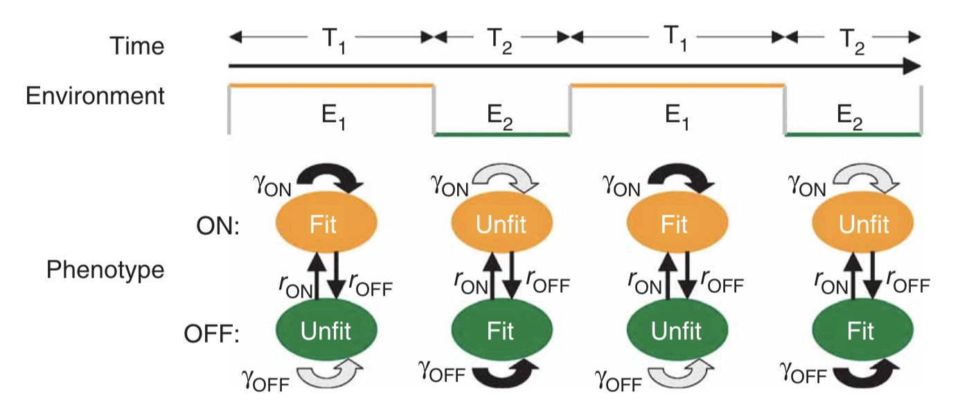
Thattai and van Oudenaarden, (Genetics, 2003) considered a minimal case in which cells can switch between two distinct states, each optimized for growth in one of two possible environments. They assumed that both the environment and the cells switch stochastically between their respective states. However, the cell is assumed not to directly sense the environment it is in. The situation here is loosely analogous to the Kelly betting example described above. You (the cell) know something about the probabilities of different environments, but not when the environment will switch. You can “bet” only by adjusting your own chances of switching between states.
In a subsequent paper, Acar et al, (Nature Genetics, 2008), the same group constructed an experimental realization of these conditions in yeast. This system took advantage of the fact that the galactose utilization circuit in yeast contains a positive feedback loop that produces two metastable states – a more complex version of the positive autoregulatory circuits we have examined previously. Cells were observed to switch stochastically between these two states. Further, by varying the concentration of galactose in the media and the expression level of a key protein in the circuit, the authors were able to engineer two different strains that both showed stochastic switching, except at distinct rates.
A minimal two-state system, fromAcar et al, Nature Genetics, 2008; Figure 1a.
If the cells simply switch randomly between states, then the key physiological parameters are the switching rates, i.e. the probability per unit time that an individual cell switches from one state to the other. If the switching rate of the cell is much faster than the switching rate of the environment, then one would tend to have a mixed population of cells, as shown in the next figure on the left. On the other hand, if the cells switch infrequently compared to the rate of environmental change then one would have the situation on the right:
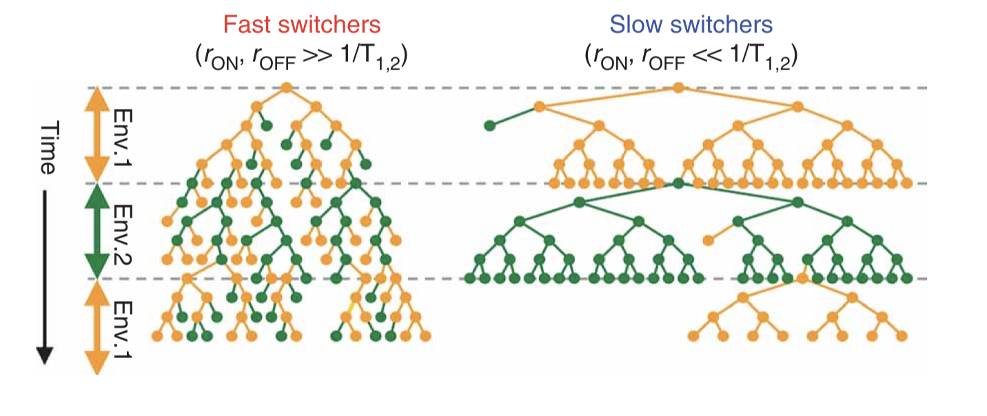
Taken fromAcar et al, Nature Genetics, 2008; Figure 1b.
The most basic question one can ask about such a system is: Given the environmental switching rate, and the growth rate (fitness) of each state in each environment, what are the optimal cellular switching rates?
To address this question, we construct a population dynamic model. That is, we write down differential equations for the number of cells, or the number of cells in each state, rather than for the number of proteins in the cell, as we have been previously. Just as proteins can be synthesized and diluted/degraded, so too cells can proliferate and dilute/die. However, a key difference between these two levels is that the rate of proliferation (at least in the exponential growth regime, far below the ‘carrying capacity’ of the environment), is proportional to the amount of cells one already has, rather than a constant production term as we have for protein expression.
We write down a minimal model for two cellular states. For simplicity, we assume a symmetry: state 0 is equally as fit in environment 0 as state 1 is in environment 1. There are then only two (rather than four) growth rates we have to think about: the growth rate of either type of cell in its more (\(\gamma_1\)) or less (\(\gamma_0\)) fit environment. The other cellular parameters are the rates of switching from the more fit to the less fit state (\(k_0\)), or vice versa (\(k_1\)).
\begin{align} \frac{dn_0}{dt} &= \gamma_0(E) n_0 -k_1 n_0 + k_0 n_1 \\[1em] \frac{dn_1}{dt} &= \gamma_1(E) n_1 +k_1 n_0 - k_0 n_1 \end{align}
The overall growth rate, which we take to be the fitness, is calculated as the growth rate of the total population size, \(n=n_0+n_1\):
\begin{align} \gamma &= \frac{1}{n} \frac{dn}{dt} \\[1em] &=\frac {\frac{dn_0}{dt}+\frac{dn_1}{dt}}{n_0+n_1} \end{align}
Analyzing this model shows that the optimal switching rate depends, as you might expect, on the switching rates of the environment, as shown here:
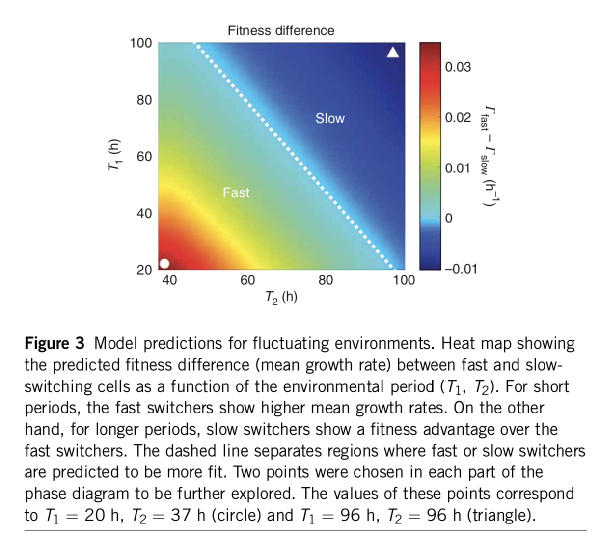
A minimal two-state system, fromAcar et al, Nature Genetics, 2008. The color scale shows the difference in predicted growth rates between fast switchers and slow switchers.
The authors conclude:
Our data suggest that tuning phenotypic switching rates may constitute a simple strategy to cope with fluctuating environments. Following this strategy, an isogenic population would improve its fitness by optimizing phenotypic diversity so that, at any given time, an optimal fraction of the population is prepared for an unforeseen environmental fluctuation. The diversity is introduced naturally through the stochastic nature of gene expression, allowing isogenic populations to mitigate the risk by ‘not putting all of their eggs in one basket’. Recent work suggests that in an adverse environment, cell-to-cell variability can have an impact on the fitness of a population29,30. Here we show that, in fluctuating environments, it is the frequency of the environmental fluctuations that constrains the inter-phenotype transition rates. In particular, we demonstrate a possible mechanism for a population to enhance its fitness in fluctuating environments by tuning the phenotypic switching rates with respect to the duration of exposures to alternating environments. This ‘resonant’ condition provides an effective survival strategy by ‘blindly’ anticipating environmental changes. This strategy could be used by cellular populations that lack dedicated signal transduction machinery for particular extracellular signals, or when it is crucial for a population to act at a faster timescale than is possible by signal transduction.
Stochastic switching can thus be a good strategy when cells are unable to detect the environment or detect it fast enough. But could it still be advantageous for a cell that can detect the environment directly?
An analytical approach enables comparison of responsive and stochastic switching strategies
Kussell and Leibler approached this problem in a general, elegant paper (Science, 2005).
The authors compare responsive and stochastic switching strategies.
Environment dynamics. They imagine a set of different environments, each of which lasts for a random, exponentially distributed, time, followed by a transition to another environmental state. The \(i^{th}\) environment has a mean lifetime, \(\tau_i\). They further allow a probabilistic alternation among environments, characterized by a matrix of environment switching rates, with \(b_{ij}\) denoting the probability of switching to environment \(i\) from environment \(j\). While each environment has some characteristic duration, and some likelihood of switching to each other environment, the exact sequence of environments experienced by any given cell is random.
Cell state dynamics On the cellular side, they similarly allow a parallel set of distinct physiological states or phenotypes, each of which can, in general, have a specific growth rate in each of the environments. A matrix, \(H_{ij}^k\) describes the rate at which cellular state \(j\) switches to cellular state \(i\) in environment \(k\).
For stochastic switching, the \(H_{ij}\) values are independent of the environment because, by definition, the cell is simply ignoring the environment.
For responsive switching, the cell can “deliberately” switch to the optimal state in each environment. Without loss of generality, one can choose the fastest growing state in environment \(k\) to be the \(k^{th}\) state. One can then write that \(H_{kj}^{(k)} = H_m\), where \(H_m\) is a single switching rate, when \(j\ne k\), with all the other \(H_{ij}^{k}\) values set to 0. In other words, everyone tries to switch to the best (\(k^{th}\)) state in each environment.
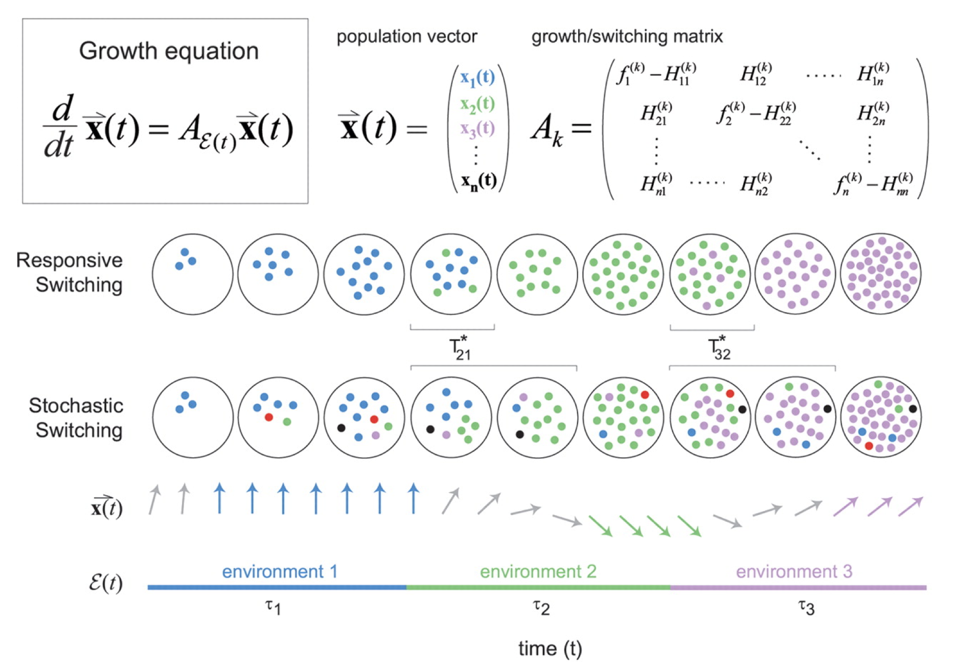
Figure taken fromKussell and Leibler, Science, 2005.
The dynamics are then described by a set of equations for the size of each cell state population, collected together in a cellular state vector, \(\mathbf{x}\). The dynamics of \(\mathbf{x}\) depend in turn on the environments, the switching rates, and the growth rates of each cell state in each environment, all collected together into the matrix \(\mathbf{A_k}\) as shown in the diagram above.
\begin{align} \frac{\mathrm{d}\mathbf{x}}{\mathrm{d}t} = \mathbf{A_k} \mathbf{x} \end{align}
Each strategy incurs a different type of cost:
Sensing requires a constant cost in the production of the sensing machinery, which is not “paid” by the stochastic switchers.
The stochastic switching strategy incurs a “diversity cost”, due to populating sub-optimal states in each environment.
They derive expressions for the growth rates in the two strategies:
Responsive switching: Long-term growth = Fastest growth - sensing cost - delay time cost
Stochastic switching: Long-term growth = Fastest growth - diversity cost - delay time cost
Note the different costs that are incurred in the two strategies. Generally speaking, sensing is favored when the diversity costs would be high, sensing costs are low, and the environment is highly variable. By contrast, stochastic switching can be favored in regimes in which sensing costs are higher, and environments are stable over longer times. (These statements are made mathematically precise in the paper).
With these general ideas in mind, we will now turn to a fascinating and biomedically important phenomenon: antibiotic persisentece.
Antibiotic persistence: a stochastic switching strategy
When one adds antibiotics to a bacterial culture, they often kill almost, but not quite, all of the cells. A small fraction of cells survive. One explanation might be the occurrence of antibiotic resistant mutants – cells that have acquired heritable mutations making them insensitive to the antibiotic. But these cells turn out not to be resistant mutants. The way to see that is to grow them up in media lacking the antibiotic, and then again expose them to antibiotic again. If they were resistant, then all of this re-grown culture would survive. With persisters, however, one finds that the antibiotic again kills the vast majority of cells, with only the same tiny fraction again surviving.
Here is a definition of persistence from Allison et al. (Current Opinion in Microbiology, 2011):
Bacterial persistence is a phenomenon in which a sub-population of cells survives antibiotic treatment…. In contrast to resistant bacteria, persisters do not grow in the presence of antibiotics and their tolerance arises from physiological processes rather than genetic mutations… Persistence was first described by Joseph Bigger in 1944 while attempting to sterilize cultures of pathogenic Staphylococcus aureus with penicillin. He found that a small number of cells “persisted” and could later form colonies even after treatment with high antibiotic concentrations.
Persistence is a major problem in many infectious diseases:
Persistence leads to recurrent infections
It extends duration of treatments
It plays an important role in the therapy choice for immunocompromised patients.
It is important for understanding infections poorly controlled by the immune system, such as tuburculosis.
Persistence is not specific to bacteria. A similar phenomenon allows cancer cells to survive chemotherapeutics. For a recent review, see: Maisonneuve and Gerdes (Cell, 2014).
The general phenomenon is diagrammed here:
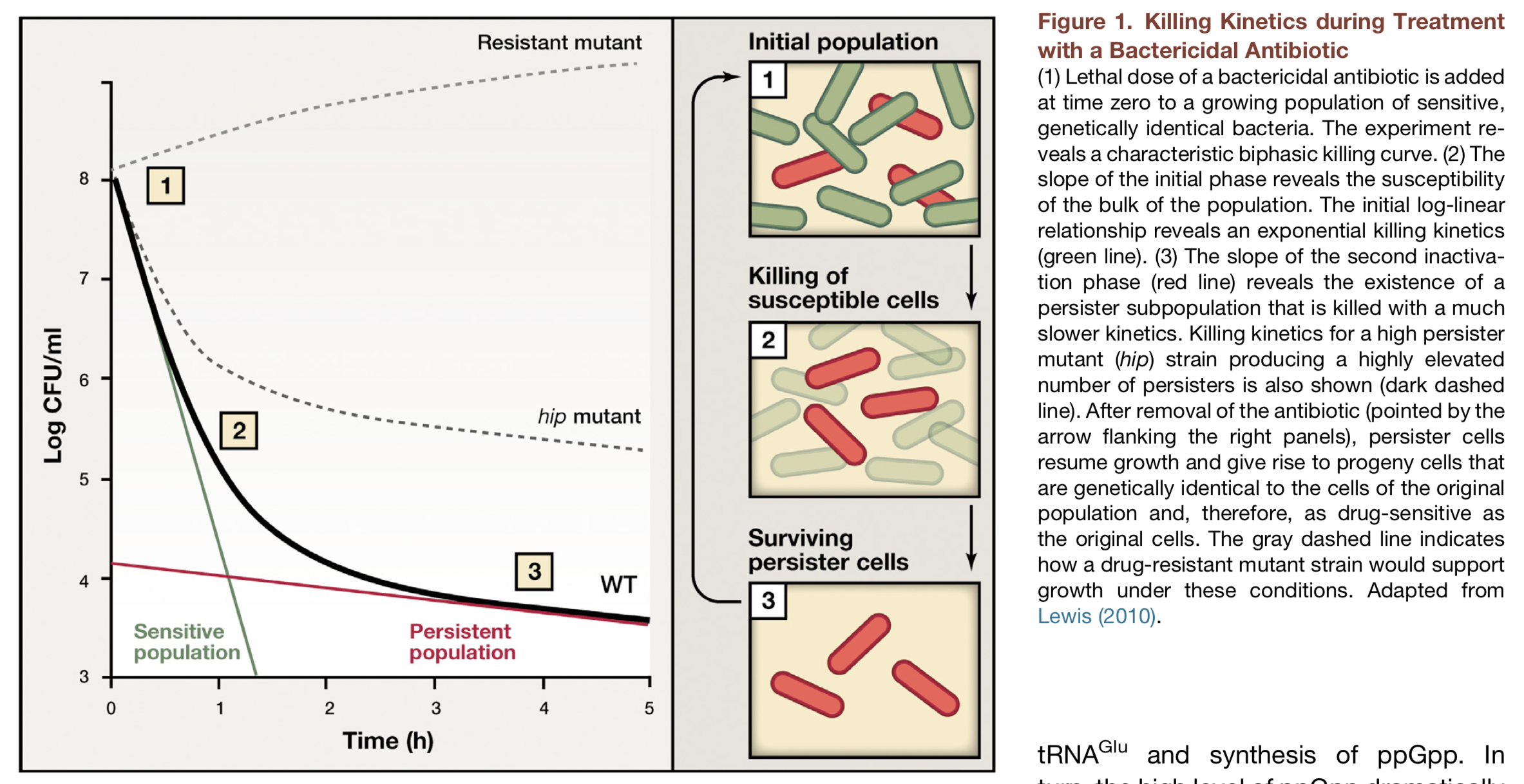
Figure taken fromMaionneuve and Gerdes, Cell, 2014.
There are different potential explanations for persistence:
Spatial heterogeneity: maybe some cells are clumped together and therefore less vulnerable to the antibiotic.
Temporal heterogeneity: perhaps adapt to the antibiotic, but do so at different rates, with only the fastest surviving.
Pre-existing heterogeneity: cells may switch among distinct, physiological states even in the absence of the antibiotic, with a small percentage occupying a transient, insensitive state at the time of antibiotic addition.
Persistence in movies
The most direct way to visualize persistence is to look at it directly using time-lapse movies. Notice here the large variation in the time at which different cells start growing, even though they are all in essentially the same environment.
Balaban and Leibler (Science, 2004) used a microfluidic approach to film cells before, during, and after antibiotic treatment. The idea was to see whether the persistent state was already present prior to the antibiotic, or whether it was a response, in some cells, to antibiotic addition.

Figure taken fromBalaban and Leibler, Science, 2004.
In this device, a predecessor to the mother machine we saw in a previous lesson, bacteria can grow in long channels embedded in PDMS, while media conditions can be rapidly changed. Using this device, one can then watch cells grow before, during, and after addition of an antibiotic, in this case ampicillin:
Here is their diagram of what they saw in the movie:
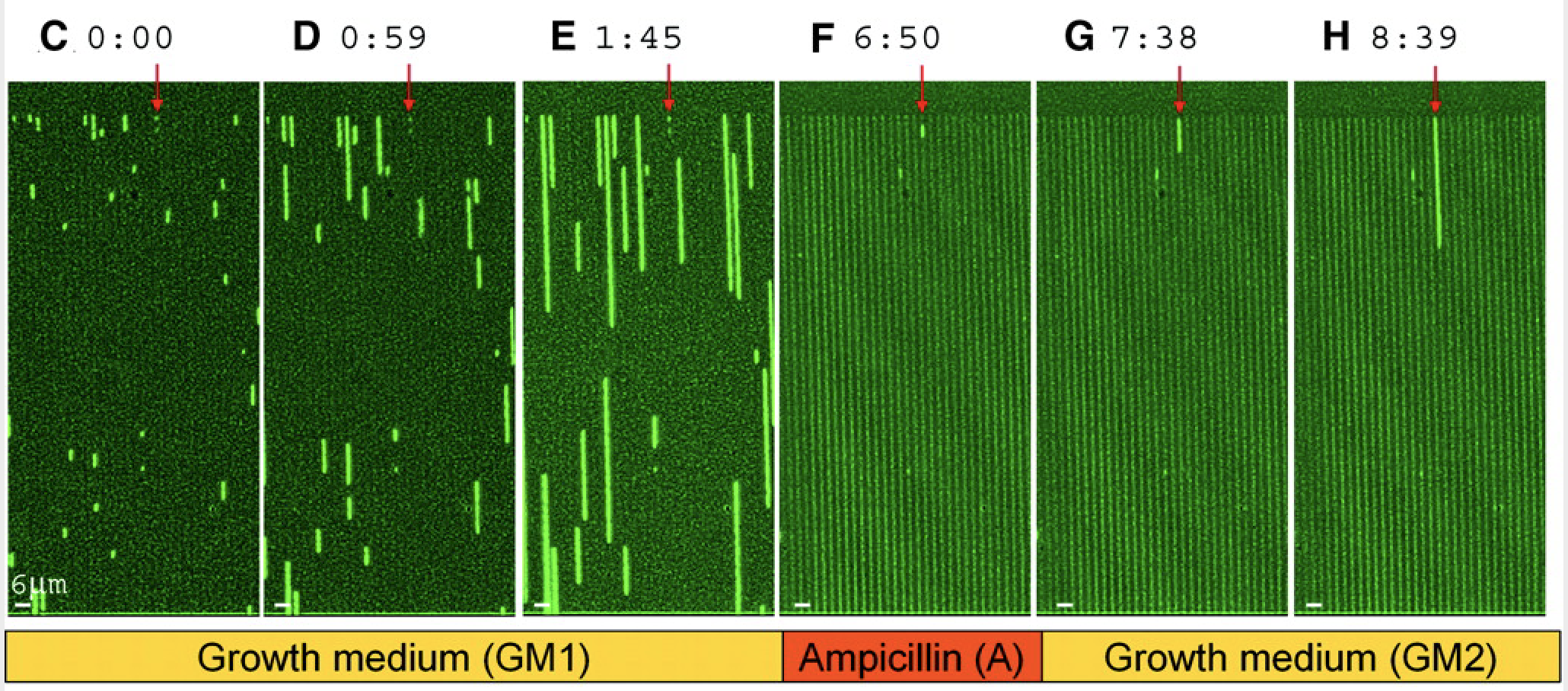
Figure taken fromBalaban and Leibler, Science, 2004.
From these experiments, we can see directly that cells spontaneously switch to persistent states characterized by slow growth. These states are far less vulnerable to attack by ampicillin, which affects cell wall synthesis. After removal of antibiotics, these cells can resume growth.
Persistence comes in multiple flavors
Through the movies and many other experiments, the authors identified two types of persisters: Those that are formed in response to a triggering event, termed type I persisters, and those that are formed spontaneously, even in constant conditions, and even in the absence of the drug, termed type II persisters. They summarized the two types of behavior with this diagram:
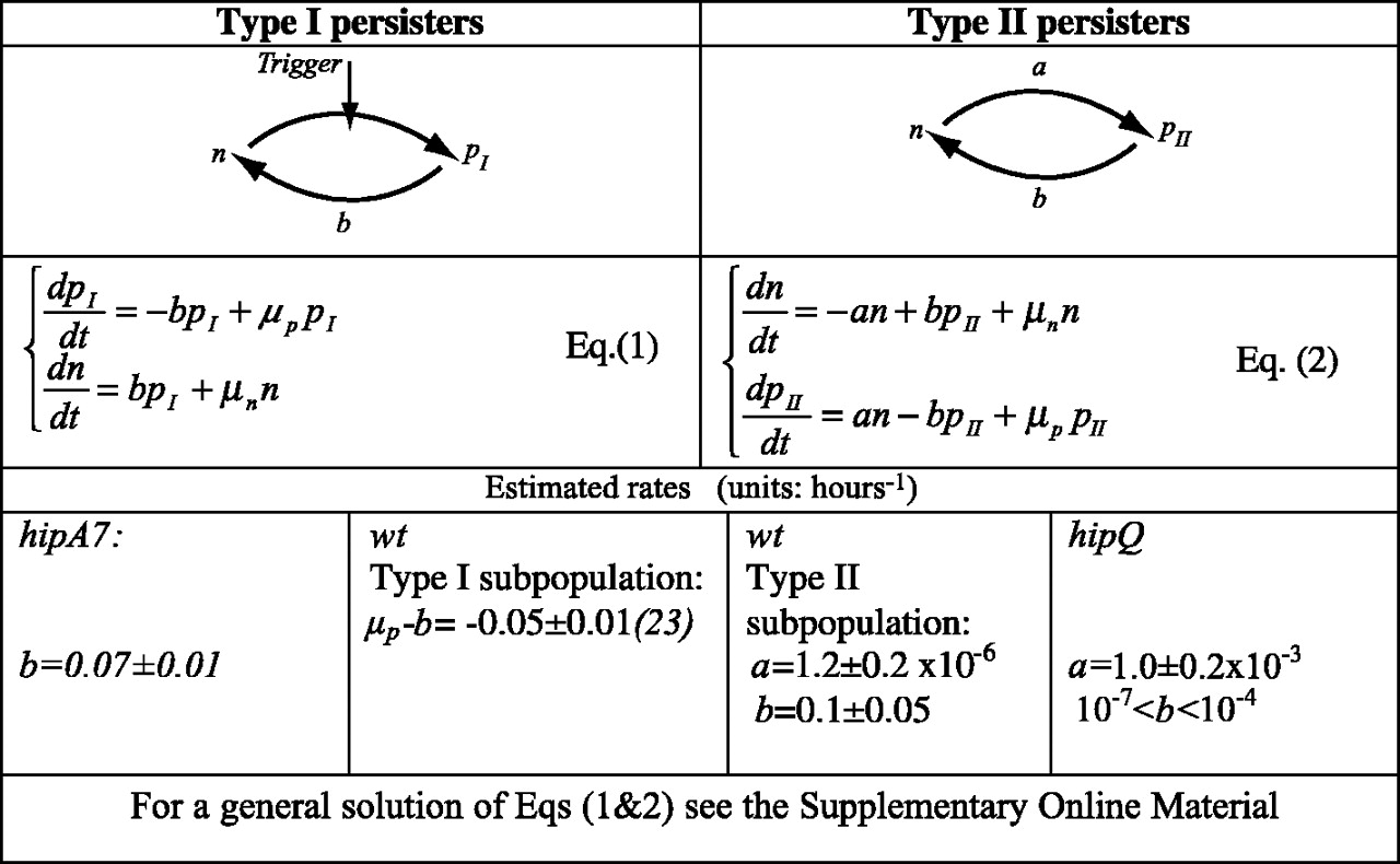
Figure taken fromBalaban and Leibler, Science, 2004.
Type I persisters are formed at stationary phase, but not during exponential growth, unlike type II persisters, which form spontaneously even in exponentially growing cultures. From the experiments, they were also able to measure the effective transition rates, as shown above, both for wild-type cells and for so-called “hip” (high incidence of persisters) mutants that generate persisters at elevated frequencies. Interestingly, the two types of persisters do not differ only in the way in which they are generated. It also appeared that type II persisters are not fully growth arrested but rather still grow, albeit an order of magnitude more slowly than normal cells.
A “toxin-antitoxin” module generates persisters through molecular titration
So far, we have seen that probabilistic “bet-hedging” strategies can be advantageous under some conditions, with antibiotic persistence providing an ideal example of such a strategy. But how is persistence implemented by underlying molecular circuits? In the previous lecture on competence, we learned that a noise-excitable circuit could generate probabilistic and transient differentiation events. The hip persistence system uses a different mechanism based on a toxin-antitoxin module. A thorough recent review of this fascinating topic can be found here.
Toxin-antitoxin modules usually consist of a two gene operon. One gene codes for a toxic protein that inhibits cell growth. The other codes for an antitoxin that binds to and inhibits the first protein. In some cases, the toxin is more stable than the antitoxin. Many naturally occurring plasmids (circular, self-replicating DNA molecules) contain such toxin-antitoxin modules. If the plasmid is lost from a cell, the antitoxin rapidly degrades, leaving the toxin, and thereby killing the cell. In this way, the plasmid ensures that once it enters a cell, none of that cells descendants can survive without it. While prevalent on plasmids, toxin-antitoxin modules also appear on bacterial chromosomes. Mycobacterium tuberculosis has 50 of them! Because they are thus able to ensure their own survival without necessarily providing any benefit to the organism, they were often thought to represent “selfish” genetic elements.
However, it appears that one function of these modules is generating stochastic episodes of persistence. In these cases, the role of the toxin protein is not to kill the cell but rather to slow or arrest its growth, reducing the cells susceptibility to antibiotics. Work on the hip system has revealed a simple molecular circuit that explains persistence.
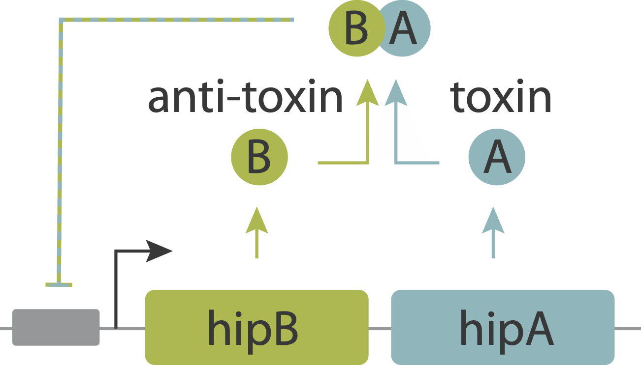
In this system, the toxin, hipA, and the antitoxin, hipB, are expressed from a single operon. The two proteins form a complex that negatively autoregulates their own expression. Because the two proteins associate very tightly they operate in a molecular titration regime in which the the anti-toxin effectively “subtracts away” toxin molecules. The excess of HipA proteins over HipB proteins represents the amount of active toxin. At high enough levels, this free HipA can trigger a dormant, growth-arrested state. Cells exit from this state after long and broadly distributed lag times of hours to days.
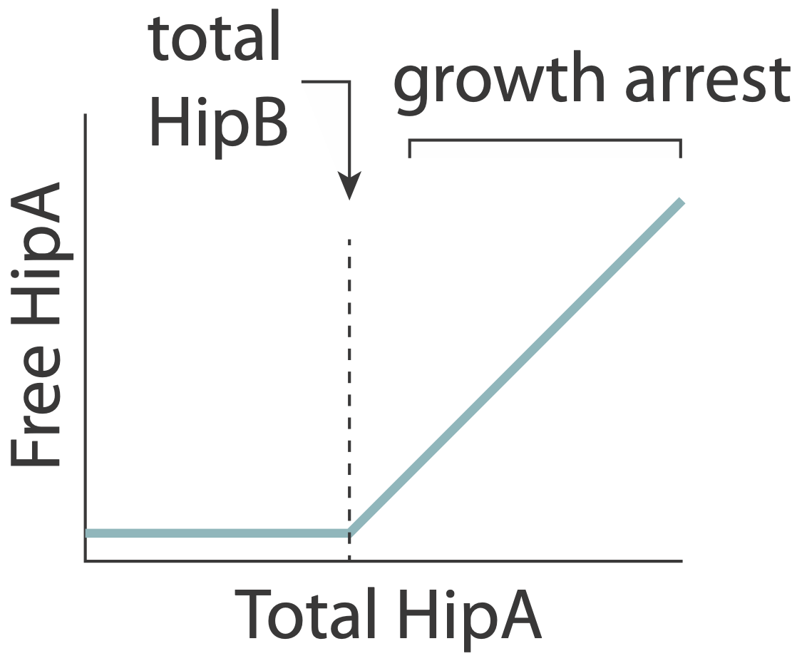
A key prediction of this model is that varying HipB levels should tune the fraction of cells that enter the dormant state. More HipB should generate fewer persisters, and vice versa. By independently regulating HipB in cells, Nathalie Balaban and colleagues experimentally demonstrated that this is indeed the case. In a stochastic model, they further showed that for reasonable parameter values, stochastic fluctuations in the levels of the two proteins could generate subpopulations of cells in which HipA exceeds HipB, triggering persistent growth-arrested states.
We will investigate molecular titration systems in more depth in an upcoming lecture.
Summary
When future outcomes are unpredictable, organisms must make “bets.”
Proportional betting provides a simple example where we can understand an optimal betting strategy.
Bacteria bet by devoting different fractions of the population to different states, each optimized for different potential environments.
Stochastic switching can outperform a sense and respond system when there are high sensing costs and low diversity costs.
Bacterial persistence represents a biomedically important natural bet-hedging system. Persisters can form prior to antibiotic exposure, and enable survival of antibiotic treatments.
Toxin-antitoxin cassettes provide a mechanism for ultra sensitive noise-driven switching between persistent and sensitive states.
Computing environment
[5]:
%load_ext watermark
%watermark -v -p numpy,bokeh,jupyterlab,biocircuits
CPython 3.7.7
IPython 7.13.0

numpy 1.18.1
bokeh 2.0.2
jupyterlab 1.2.6
biocircuits 0.0.16