13. Stochastic differentiation
Design principles
Fast positive feedback combined with slow negative feedback can combine to give excitable circuits.
Concepts
Excitable circuits have a unique, globally attracting rest state and a large stimulus can send the system on a long excursion before it returns to the resting state.
Techniques
Plots of phase portraits.
[1]:
import collections
import tqdm

import pandas as pd
import numpy as np
import scipy.integrate
import numba

import biocircuits

import bokeh.io
import bokeh.plotting

import colorcet
import bokeh_catplot

bokeh.io.output_notebook()
Note: To run this notebook, you will need to update the biocircuits package, which can be done by doing pip install --upgrade biocircuits on the command line.
Noise: A bug or feature?
In the past two lessons, we have studied noise, how it comes about, how to quantify it, and how to take it into account when we study the dynamics of biological circuits. Noise is certainly a part of biological circuits, but is noise a bug for a feature?
We often regard noise as an unavoidable nuisance in biological life, especially at the scale of an individual cell. Perhaps we have this view because noise, by design, is generally absent from electronic circuits, which operate essentially deterministically. But perhaps noise could provide functional enabling capabilities for cells and organisms. If so, we can think about what these capabilities may be, and further how they are implemented by the circuits.
Excitability as a property of a dynamical system
We have seen seen several properties of dynamical systems enable cellular capabilities. Examples are in the table below.
Dynamical system property |
Cellular capability |
|---|---|
Monostable fixed point |
Remain in a constant state |
Bistability |
Exist in multiple epigenetically stable states (e.g., toggle switch) |
Limit cycles |
Ability to maintain oscillations (e.g., repressilator) |
In this lesson, we will discuss how another property of dynamical systems, that of excitability, may be used to enable probabilistic and transient differentiation events. We will discuss this in the context of cellular competence, which we discuss in the next section.
Excitability is tricky to define. Borrowing from Strogatz (in Nonlinear Dynamics and Chaos) an excitable system has two key properties:
It has a unique, globally attracting rest state;
A large enough stimulus can send the system on a long excursion before it returns to the resting state.
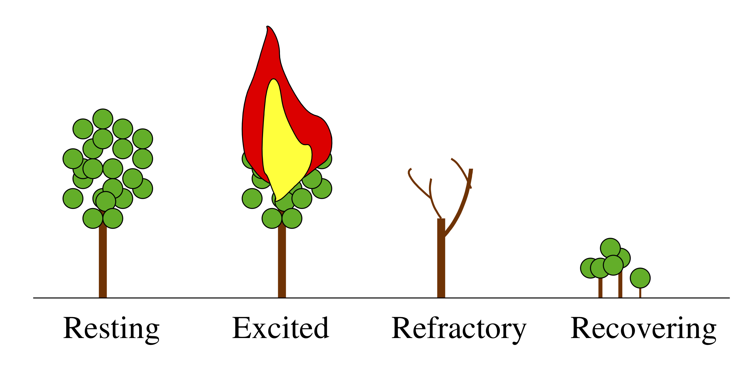
A forest is a classic example of an excitable system. Its resting state consists of many trees peacefully photosynthesizing and providing shade for hikers. Occasionally, though, an errant lightning strike or a careless camper can perturb the system on a large excursion wherein the forest burns, recovers, and then grows back again.
The membrane potentials of neurons are also excitable systems. When resting, they sit at their postsynaptic potential (PSP) and a stimulus results in them relaxing immediately back to their PSP. However, when they are excitable, a stimulus and lead to a big excursion wherein the membrane potential grows far beyond the PSP, before returning back to the PSP. This excursion is called a spike.
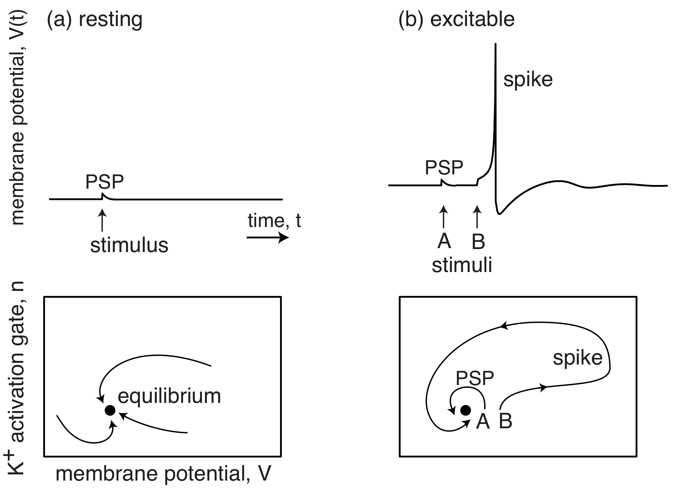
(Image adapted from Izhikevich, Dynamical Systems in Neuroscience, 2007.)
Importantly, stochastic fluctuations can be the source of the perturbation that pushes an excitable circuit off on one of its excursions.
Cellular competence
When stressed, bacterial species, like Bacillus subtilis, have several responses.
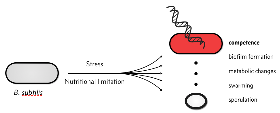
In particular, they can become competent, which means that they can take up environmental DNA. There is plenty of speculation as to the evolutionary advantage of competence, but we will not discuss that here. Rather, we will discuss the circuit governing how B. subtilis cells switch between a non-competent state, called a vegetative state to a competent one.
The response of individual cells to a stress is heterogeneous; some cells sporulate, some remain vegetative, some become competent, some die, etc.
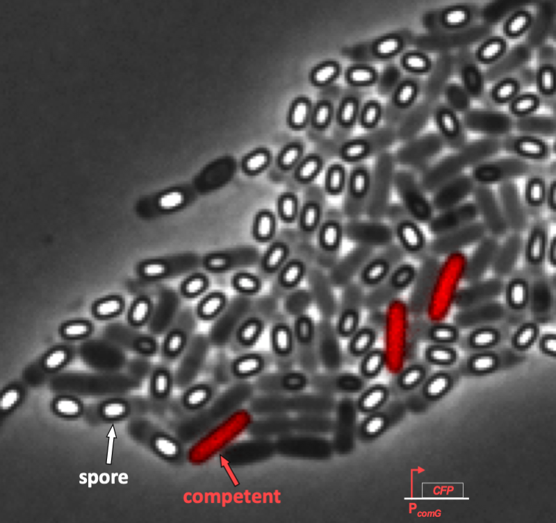
We can see this even more clearly in time lapse video. As we will discuss in a moment when we introduce the circuit responsible for competence, competent cells show up as pink/purple in the movie below.
In the video, it is evident that competence is both probabilistic (only a few cells become competent) and transient (competence is a temporary condition). These are hallmarks of excitability, and we will not examine the genetic circuit responsible for this excitability. In particular, we see to address the following questions.
How do cells enter and exit competence?
How do cells regulate the frequency and duration of competence?
Can these properties be tuned?
Is noise necessary to induce competence?
The B. subtilis competence circuit
The genetic circuit responsible for competence is connected to receptors responsible for sensing the environment and other circuits within the cell. The result can be a bit complicated, as shown in the figure below.
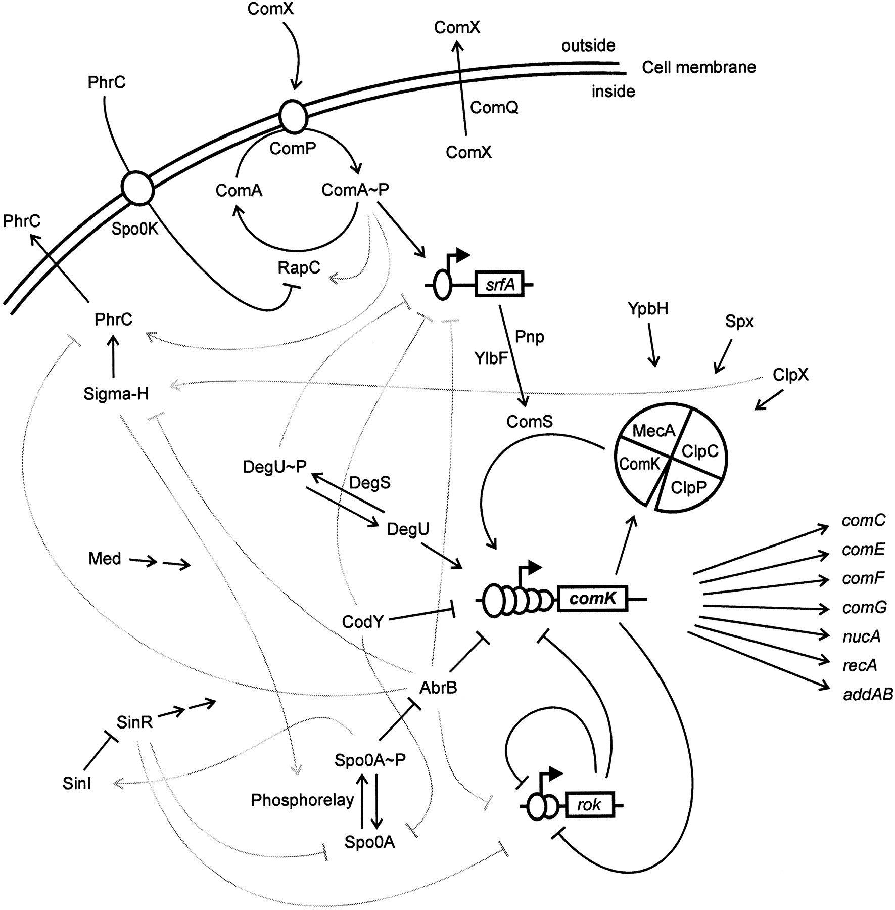
Image taken from Hamoan, et al., Microbiology, 2003
At the core of the circuit is ComK, which is necessary and sufficient for differentiation into competence. A simplified circuit, focusing on this ComK core, taken from Süel, et al., Nature, 2006, is shown below.
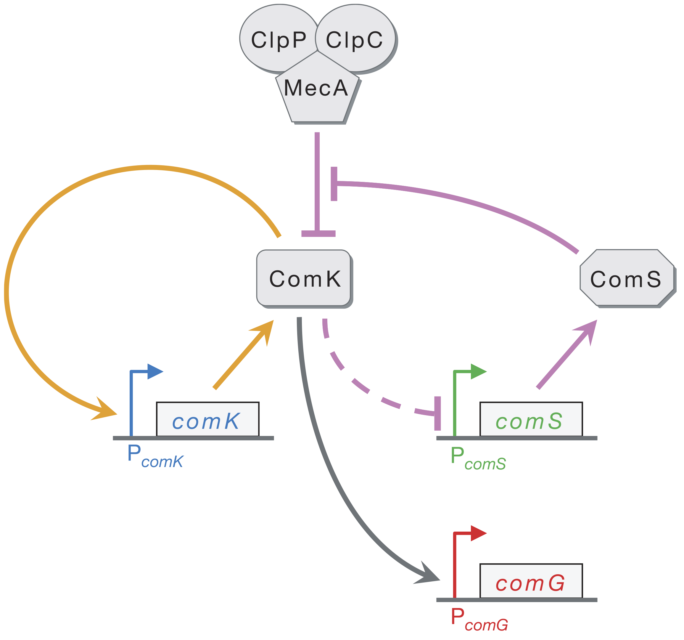
ComK activates its own transcription in a positive feedback loop (orange). ComK indirectly represses ComS (as marked by the dashed line). ComK is also degraded by the MecA–ClpP–ClpC complex (which we will call MecA for short), but so is ComS. This competition for degradation by MecA effectively means that ComS inhibits degradation of ComK by MecA. Finally, ComG is one of the genes activated by ComK that result in competence.
Süel and coworkers inserted pairwise combinations of the promoters for comK, comG and comS expression YFP and CFP in B. subtilis to monitor the levels of those genes. This is why the competent cells appeard purple in the movie above; both ComK (blue channel) and ComG (red channel) are active in competent cells.
We can look at the circuit to reason how it might be excitable. Imagine there is a transient excitement of ComK levels. This excitement is amplified by positive feedback (the orange arrows), leading to more production of ComK. There is enough ComS around to keep MecA from degrading the ComK molecules that are made due to the positive feedback. On a longer time scale, however, production of ComS gets inhibited, which results in the MecA complex starting to degrade ComK instead of ComS. This brings ComK back to its pre-excitedment level. In this sense, ComS serves to help initiate competence by reducing degradation of ComK, but also serves to bring the exit of competence when it is repressed by the excessive ComK.
This leads to a design principle. Fast positive feedback combined with slow negative feedback can combine to give excitable circuits.
In what follows, we will explore this competence circuit in more detail to get a quantitative understanding of how it works.
A model for the ComK circuit
To model the ComK circuit, we will follow the logic of Süel, et al. (Science, 2007). The MecA complex degrades ComK and ComS. ComS serves to inhibit this degradation by tying up the MecA complex in degrading itself. That is, there are two competing reactions: degradation of ComK and degradation of ComS. We take both of these reaction to have Michaelis-Menten kinetics, giving the reaction schemes
\begin{align} &\text{MecA} + \text{ComK} \stackrel{\gamma_{\pm a}}{\rightleftharpoons} \text{MecA-ComK} \stackrel{\gamma_1}{\rightarrow} \text{MecA} \\[1em] &\text{MecA} + \text{ComS} \stackrel{\gamma_{\pm b}}{\rightleftharpoons} \text{MecA-ComS} \stackrel{\gamma_2}{\rightarrow} \text{MecA}. \end{align}
ComK is also known to indirectly inhibit expression of ComS, denoted by the dashed arrow. We take this to be described by a Hill function. Finally, ComK has a basal expression level. We can therefore write the dynamical equations for ComK and the MecA-ComK complex as
\begin{align} \frac{\mathrm{d}K}{\mathrm{d}t}&= \alpha_k + \beta_k\,\frac{K^n}{k_k^n + K^n} - \gamma_a M_f K + \gamma_{-a}M_K - \gamma_k K,\\[1em] \frac{\mathrm{d}M_K}{\mathrm{d}t} &= -(\gamma_{-a} + \gamma_1)M_K + \gamma_aM_f K, \end{align}
where we have denoted the concentration of MecA-ComK as \(M_K\) and of free MecA as \(M_f\). We have also assumed that ComK undergoes non-catalyzed degradation, characterized by degradation rate \(\gamma_k\).
We write the influence of ComK on ComS expression as a repressive Hill function. With our assumption of Michaelis-Menten kinetics on ComS degradation by MecA, we can now write the dynamical equations for ComS and the ComS-MecA complex.
\begin{align} \frac{\mathrm{d}S}{\mathrm{d}t}&= \frac{\beta_s}{1 + (K/k_s)^p} - \gamma_b M_f S + \gamma_{-b}M_S - \gamma_s S,\\[1em] \frac{\mathrm{d}M_S}{\mathrm{d}t} &= -(\gamma_{-b} + \gamma_2)M_S + \gamma_b M_f S. \end{align}
Now, if we assume that the conversion of the MecA-Com complexes are very fast (\(\gamma_1\) and \(\gamma_2\) are large), we can make a pseudo-steady state approximation such that \(\mathrm{d}M_K/\mathrm{d}t \approx \mathrm{d}M_S/\mathrm{d}t \approx 0\). Finally, if we assume that the total amount of MecA complex is conserved, i.e., \(M_f + M_K + M_S = M_\mathrm{total} \approx \text{constant}\), we can simply our expressions. Specifically, we now have
\begin{align} \frac{\mathrm{d}K}{\mathrm{d}t}&= \alpha_k + \beta_k\,\frac{K^n}{k_k^n + K^n} -\gamma_1M_K - \gamma_k K,\\[1em] \frac{\mathrm{d}S}{\mathrm{d}t}&= \alpha_s + \frac{\beta_s}{1 + (K/k_s)^p} - \gamma_2 M_S - \gamma_s S. \end{align}
We can get expressions for \(M_K\) and \(M_S\) in terms of \(M_\mathrm{total}\), \(K\), and \(S\) by using the relations following our two assumptions,
\begin{align} -(\gamma_{-a} + \gamma_1)M_K + \gamma_a(M_\mathrm{total} - M_K - M_S) K &= 0,\\[1em] -(\gamma_{-b} + \gamma_2)M_S + \gamma_b(M_\mathrm{total} - M_K - M_S) S &= 0. \end{align}
We can write these in a more convenient form to eliminate \(M_K\) and \(M_S\).
\begin{align} (\gamma_{-a} + \gamma_1 + \gamma_a K)M_K + \gamma_a K M_S &= \gamma_a M_\mathrm{total} K \\[1em] \gamma_b S M_K + (\gamma_{-b} + \gamma_2 + \gamma_b S)M_S &= \gamma_b M_\mathrm{total} S. \end{align}
Solving this system of linear equations for \(M_K\) and \(M_S\) yields
\begin{align} M_K &= M_\mathrm{total}\,\frac{K/\Gamma_k}{1 + K/\Gamma_k + S/\Gamma_s}, \\[1em] M_S &= M_\mathrm{total}\,\frac{S/\Gamma_s}{1 + K/\Gamma_k + S/\Gamma_s}, \end{align}
where \(\Gamma_k \equiv (\gamma_{-a} + \gamma_1)/\gamma_a\) and \(\Gamma_k \equiv (\gamma_{-b} + \gamma_2)/\gamma_b\). Inserting these expressions back into our ODEs for the \(K\) and \(S\) dynamics and defining \(\delta_k\equiv \gamma_1 M_\mathrm{total}/\Gamma_k\) and \(\delta_s \equiv\gamma_2 M_\mathrm{total}/\Gamma_s\) for notational convenience yields
\begin{align} \frac{\mathrm{d}K}{\mathrm{d}t}&= \alpha_k + \beta_k\,\frac{K^n}{k_k^n + K^n} - \frac{\delta_k K}{1 + K/\Gamma_k + S/\Gamma_s} - \gamma_k K\\[1em] \frac{\mathrm{d}S}{\mathrm{d}t}&= \alpha_s + \frac{\beta_s}{1 + (K/k_s)^p} - \frac{\delta_s S}{1 + K/\Gamma_k + S/\Gamma_s} - \gamma_s S. \end{align}
We will nondimensinalize time by the rate of ComK degradation by the MecA complex, \(\delta_k\). The parameters \(\Gamma_k\) and \(\Gamma_s\) are natural choices for nondimensionalizing \(K\) and \(S\). The resulting dimensionless equations are
\begin{align} \frac{\mathrm{d}k}{\mathrm{d}t}&= a_k + \frac{b_k\,(k/\kappa_k)^n}{1 + (k/\kappa_k)^n} - \frac{k}{1 + k + s} - \gamma_k k, \\[1em] \frac{\mathrm{d}s}{\mathrm{d}t}&= a_s + \frac{b_s}{1 + (k/\kappa_s)^p} - \frac{s}{1 + k + s} - \gamma_s s. \end{align}
It is left to the reader to work out the relationships between the dimensionless and dimensional parameters.
Analysis of the dynamical system
Now that we have our dynamic system set up, we can begin analysis. We will start by defining parameters for the system, using the parameters specified in the Süel, et al. paper. For convenience, we will store the parameters in a container.
[2]:
CompetenceParams = collections.namedtuple(
    "CompetenceParams",
    [
        "a_k",
        "a_s",
        "b_k",
        "b_s",
        "kappa_k",
        "kappa_s",
        "gamma_k",
        "gamma_s",
        "n",
        "p",
    ],
)

params = CompetenceParams(
    a_k=0.00035,
    a_s=0.0,
    b_k=0.3,
    b_s=3.0,
    kappa_k=0.2,
    kappa_s=1 / 30,
    gamma_k=0.1,
    gamma_s=0.1,
    n=2,
    p=5,
)
With the parameters in hand, we can define the time derivatives for the dimensionless ComK and ComS concentrations.
[3]:
def dk_dt(k, s, p):
    """p is a CompetenceParams instance"""
    return (
        p.a_k
        + p.b_k * k ** p.n / (p.kappa_k ** p.n + k ** p.n)
        - k / (1 + k + s)
        - p.gamma_k * k
    )


def ds_dt(k, s, p):
    return (
        p.a_s
        + p.b_s / (1 + (k / p.kappa_s) ** p.p)
        - s / (1 + k + s)
        - p.gamma_s * s
    )
We have seen that plotting the nullclines is a useful exercise, as this exposes the fixed points. This this system, the nullclines are most easily represented in for form \(s(k)\), that is, \(s\) as a function of \(k\). These are easily derived by setting \(\mathrm{d}k/\mathrm{d}t\) and \(\mathrm{d}s/\mathrm{d}t\) equal to zero.
\begin{align} &\frac{\mathrm{d}k}{\mathrm{d}t} = 0 \;\Rightarrow s\; = \frac{k}{a_k - \gamma_k k + b_k k^n / (\kappa_k^n + k^n)} - k - 1. \end{align}
The nullcline given by \(\mathrm{d}s/\mathrm{d}t = 0\) is the positive root of the quadratic polynomial equation \(as^2 + b s + c = 0\) with
\begin{align} a &= \gamma_s,\\[1em] b &= 1 + \gamma_s(1+k) - A,\\[1em] c &= -A(1+k), \end{align}
with
\begin{align} A = a_s + \frac{b_s}{(1 + (k/\kappa_s)^p}. \end{align}
We can code these up.
[4]:
def k_nullcline(k, p):
    abk = (
        p.a_k
        + p.b_k * k ** p.n / (p.kappa_k ** p.n + k ** p.n)
        - p.gamma_k * k
    )
    return k / abk - k - 1


def s_nullcline(k, p):
    A = p.a_s + p.b_s / (1 + (k / p.kappa_s) ** p.p)
    a = p.gamma_s
    b = 1 - A + p.gamma_s * (1 + k)
    c = -A * (1 + k)

    return -2 * c / (b + np.sqrt(b ** 2 - 4 * a * c))
We will being our graphical analysis by plotting the nullclines, as we have done in past lessons. Knowing what our demands will be in a moment when plotting the phase portrait, we will write a function to plot the nullclines where the \(k\) and \(s\) axes are on a logarithmic scale and also on a linear scale.
[5]:
def plot_nullclines(k_range, s_range, params, log=True, p=None, **kwargs):
    """
    Compute and plot the nullclines.
    """
    if log:
        x_range = np.log10(k_range)
        y_range = np.log10(s_range)
    else:
        x_range = k_range
        y_range = s_range

    if p is None:
        p = bokeh.plotting.figure(
            frame_width=260,
            frame_height=260,
            x_axis_label="log₁₀ k",
            y_axis_label="log₁₀ s",
            x_range=x_range,
            y_range=y_range,
            **kwargs
        )

    def filter_out_of_range(k, s_nck, s_ncs):
        k_k = k.copy()
        k_s = k.copy()
        inds_k = np.logical_or(s_nck < s_range[0], s_nck > s_range[1])
        inds_s = np.logical_or(s_ncs < s_range[0], s_ncs > s_range[1])
        s_nck[inds_k] = np.nan
        s_ncs[inds_s] = np.nan
        k_k[inds_k] = np.nan
        k_s[inds_s] = np.nan

        return k_k, k_s, s_nck, s_ncs


    if log:
        k = np.logspace(np.log10(k_range[0]), np.log10(k_range[1]), 200)
        s_nck = k_nullcline(k, params)
        s_ncs = s_nullcline(k, params)
        k_k, k_s, s_nck, s_ncs = filter_out_of_range(k, s_nck, s_ncs)
        p.line(np.log10(k_k), np.log10(s_nck), color="#ff7f0e", line_width=3)
        p.line(np.log10(k_s), np.log10(s_ncs), color="#9467bd", line_width=3)
    else:
        k = np.linspace(k_range[0], k_range[1], 200)
        s_nck = k_nullcline(k, params)
        s_ncs = s_nullcline(k, params)
        k_k, k_s, s_nck, s_ncs = filter_out_of_range(k, s_nck, s_ncs)
        p.line(k_k, s_nck, color="#ff7f0e")
        p.line(k_s, s_ncs, color="#9467bd")

    return p
We can now use this function to make the plot. We will use the parameter values from the Süel, et al. paper and make the plot with \(k\) and \(s\) on a logarithmic scale. Note that we are labeling our axes as “log₁₀ k” instead of choosing x_axis_type = 'log' as a keyword argument when building the figure. Our reason for doing this will become clear when we add a phase portrait to the plot.
[6]:
k_range = np.array([1e-3, 2])
s_range = np.array([1e-3, 5000])

p = plot_nullclines(k_range, s_range, params, log=True)
bokeh.io.show(p)
The nullclines have three crossings, implying three fixed points. To investigate the behavior near the fixed point, and indeed away from them as well, we can plot the phase portrait. A phase portrait is a plot displaying possible trajectories of a dynamical system in phase space, in this case on the \(k\)-\(s\) plane. Let’s generate a phase portrait using the biocircuits package (with the nullclines overlaid) to look at one, and then we will revisit how it is generated.
[7]:
# Make the plot
p = plot_nullclines(k_range, s_range, params, log=True)

p = biocircuits.phase_portrait(
    dk_dt, ds_dt, k_range, s_range, (params,), (params,), log=True, p=p,
)

bokeh.io.show(p)
The phase portrait is intuitive. The streamlines depict how the system evolves with time. Coming from the top (lots of ComS is around), if \(k\) is small (there is not much ComK around), the system tends toward the leftmost fixed point. If \(k\) is larger, though, the system makes an excursion to large \(k\) values, and then drops to large \(k\)/low \(s\), before returning back to the leftmost fixed point. This is indeed the hallmark of an excitable system. It takes a large excursion in phase space before returning to a stable fixed point. We will refer to this excursion, which is the time the cell spends in competence, as the “competence loop.”
To better understand the dynamics close to the fixed points, we can take a closer look. The biocircuits package enables making zoomable phase portraits by using the zoomable=True kwarg. However, these plots do not render in static HTML because they require a Python engine to be running to compute the streamlines. Here is a zoomable plot if you are working in a live notebook. (The cell will show no output in the HTML version of the notebook.)
[8]:
p = plot_nullclines(k_range, s_range, params, log=True,)

p = biocircuits.phase_portrait(
    dk_dt,
    ds_dt,
    k_range,
    s_range,
    (params,),
    (params,),
    log=True,
    p=p,
    zoomable=True,
)

bokeh.io.show(p)
For static HTML rendering, we will make zoomed-in plots around the fixed points. We start with the leftmost fixed point.
[9]:
k_range = [0.0025, 0.0030]
s_range = [15, 30]

p = plot_nullclines(k_range, s_range, params, log=True)

p = biocircuits.phase_portrait(
    dk_dt, ds_dt, k_range, s_range, (params,), (params,), log=True, p=p,
)

bokeh.io.show(p)
This is a stable fixed point, with the system flowing into it from all directions (when \(k\) and \(s\) are close to the fixed point). Let’s now look at the fixed point for the next largest \(k\).
[10]:
k_range = [0.014, 0.02]
s_range = [10, 30]

p = plot_nullclines(k_range, s_range, params, log=True)

p = biocircuits.phase_portrait(
    dk_dt, ds_dt, k_range, s_range, (params,), (params,), log=True, p=p,
)

bokeh.io.show(p)
We can see from the flow lines that this is an unstable fixed point, a saddle. We could perform linear stability analysis on this fixed point, and we would find a positive trace and a negative determinant of the linear stability matrix, which means one eigenvalue is positive and the other is negative. This means that the system comes toward the fixed point from one direction, but is pushed away along the other.
Finally, let’s look at the last fixed point, for largest \(k\).
[11]:
k_range = [0.02, 0.05]
s_range = [1, 15]

p = plot_nullclines(k_range, s_range, params, log=True)

p = biocircuits.phase_portrait(
    dk_dt, ds_dt, k_range, s_range, (params,), (params,), log=True, p=p
)

bokeh.io.show(p)
This fixed point is a spiral source. It is unstable and spirals the system away from it.
Numerical solution of dynamical equations
Now that we have a good picture of the dynamics, we can numerically solve the dynamical equations. Of course, the initial conditions are relevant here. We will start with no ComK or ComS (which is not at all relevant physiologically) and solve.
[12]:
# Right-hand-side of ODEs
def rhs(ks, t, p):
    """
    Right-hand side of dynamical system.
    """
    k, s = ks
    return np.array([dk_dt(k, s, p), ds_dt(k, s, p)])

# Set up and solve
t = np.linspace(0, 200, 100)
ks_0 = np.array([0, 0])
ks = scipy.integrate.odeint(rhs, ks_0, t, args=(params,))
k, s = ks.transpose()
We will plot this in phase space, with the nullclines overlaid. The trajectory is in gray.
[13]:
k_range = np.array([1e-3, 2])
s_range = np.array([1e-3, 5000])

p = plot_nullclines(k_range, s_range, params, log=True)
p.line(np.log10(k[1:]), np.log10(s[1:]), line_width=2, color='gray')

bokeh.io.show(p)
We see a rise to the fixed point. Now, let’s say we had some fluctuation that kicked us up a bit off of the fixed point. We’ll start with \(s = 6\) and \(k = 0.05\) and we’ll color the trajectory in a blue color.
[14]:
# Set up and solve
t = np.linspace(0, 200, 300)
ks_0 = np.array([1e-2, 1e3])
ks = scipy.integrate.odeint(rhs, ks_0, t, args=(params,))
k2, s2 = ks.transpose()

p.line(np.log10(k2), np.log10(s2), line_width=2, color='steelblue')

bokeh.io.show(p)
The system takes a much longer trajectory to get to the fixed point, taking the excursion we suspected it would from the phase portrait.
Stochastic simulation
As we have just seen, the system can take a transient journey into competence provided it is perturbed far enough away from the stable fixed point. This raises the question, is intrinsic noise enough to give the “kick” needed to make the excursion to competence? To investigate this, we can perform a Gillespie simulation (SSA) to investigate the dynamics. To specify the master equation, we need the usual ingredients.
A definition of the species present with variables representing their copy number.
A definition of the unit moves that are allowed (the nonzero transition kernels).
Updates to copy numbers for each move.
The propensity for each move.
We can conveniently organize these in tables. First, the variables.
index |
description |
variable |
|---|---|---|
0 |
comK mRNA copy number |
|
1 |
ComK protein copy number |
|
2 |
comS mRNA copy number |
|
3 |
ComS protein copy number |
|
4 |
Free MecA complex copy number |
|
5 |
MecA-ComK complex copy number |
|
6 |
MecA-ComS complex copy number |
|
With the species defined, we an write the move set with propensities.
index |
description |
update |
propensity |
|---|---|---|---|
0 |
constitutive transcription of a comK mRNA |
|
|
1 |
regulated transcription of a comK mRNA |
|
|
2 |
translation of a ComK protein |
|
|
3 |
constitutive transcription of a comS mRNA |
|
|
4 |
regulated transcription of a comS mRNA |
|
|
5 |
translation of a ComS protein |
|
|
6 |
degradation of a comK mRNA |
|
|
7 |
degradation of a comK protein |
|
|
8 |
degradation of a comS mRNA |
|
|
9 |
degradation of a comS protein |
|
|
10 |
binding of MecA and ComK |
|
|
11 |
unbinding of MecA and ComK |
|
|
12 |
degradation ComK by MecA |
|
|
13 |
binding of MecA and ComS |
|
|
14 |
unbinding of MecA and ComS |
|
|
15 |
degradation ComS by MecA |
|
|
In defining the propensities, we introduced parameters. We can define their values, again in accordance with the Süel, et al. paper.
parameter |
value |
units |
|---|---|---|
|
1 |
– |
|
1 |
– |
|
1 |
– |
|
1 |
– |
|
1 |
molecule/nM |
|
0.00021875 |
1/sec |
|
0.1875 |
1/sec |
|
0.2 |
1/sec |
|
0 |
– |
|
0.0015 |
1/sec |
|
0.2 |
1/sec |
|
0.005 |
1/sec |
|
0.0001 |
1/sec |
|
0.005 |
1/sec |
|
0.0001 |
1/sec |
|
2.02×10\(^{-6}\) |
1/nM-sec |
|
0.0005 |
1/sec |
|
0.05 |
1/sec |
|
4.5×10\(^{-6}\) |
1/nM-sec |
|
5×10\(^{-5}\) |
1/nM-sec |
|
4×10\(^{-5}\) |
1/sec |
|
5000 |
nM |
|
833 |
nM |
|
2 |
– |
|
5 |
– |
Additionally, we take the total MecA complex copy number to be 500. That is, af+ak+as_ = 500.
If is useful to connect these parameters to those of the ODEs we have considered so far and have used to build the phase portraits. As a reminder, the dimensional version of those ODEs is
\begin{align} \frac{\mathrm{d}K}{\mathrm{d}t}&= \alpha_k + \beta_k\,\frac{K^n}{k_k^n + K^n} - \frac{\delta_k K}{1 + K/\Gamma_k + S/\Gamma_s} - \gamma_k K\\[1em] \frac{\mathrm{d}S}{\mathrm{d}t}&= \alpha_s + \frac{\beta_s}{1 + (K/k_s)^p} - \frac{\delta_s S}{1 + K/\Gamma_k + S/\Gamma_s} - \gamma_s S. \end{align}
By working through the propensities and performing some algebraic manipulations that we will not go through here (though you can on your own if you like), the parameters in the ODEs above are related to those of the discrete model as follows.
\begin{align} &\alpha_k = \frac{k_1\,k_3}{k_7}\,\frac{P_\mathrm{comK}^\mathrm{const}}{\Omega},\\[1em] &\alpha_s = \frac{k_4\,k_6}{k_9}\,\frac{P_\mathrm{comS}^\mathrm{const}}{\Omega},\\[1em] &\beta_k = \frac{k_2\,k_3}{k_7}\,\frac{P_\mathrm{comK}}{\Omega},\\[1em] &\beta_s = \frac{k_5\,k_6}{k_9}\,\frac{P_\mathrm{comS}}{\Omega},\\[1em] &\Gamma_k = \frac{k_{-11}+k_{12}}{k_{11}} \\[1em] &\Gamma_s = \frac{k_{-13}+k_{14}}{k_{13}} \\[1em] &\delta_k = \frac{k_{12}\,M}{\Gamma_k} \\[1em] &\delta_s = \frac{k_{14}\,M}{\Gamma_s} \\[1em] &\gamma_k = k_8,\\[1em] &\gamma_s = k_{10}, \end{align}
where \(M\) is the total MecA complex copy number (taken to be \(M = 500\)).
We now have all the ingredients, so we can proceed to code up the simulation. That is, we supply the propensity function and updates.
[15]:
@numba.njit
def propensity(
    propensities,
    population,
    t,
    P_comK_const,
    P_comS_const,
    P_comK,
    P_comS,
    omega,
    k1,
    k2,
    k3,
    k4,
    k5,
    k6,
    k7,
    k8,
    k9,
    k10,
    k11,
    km11,
    k12,
    k13,
    km13,
    k14,
    kappa_k,
    kappa_s,
    n,
    p,
):
    mk, pk, ms, ps, af, ak, as_ = population

    f_num = (pk / kappa_k * omega) ** n
    f = k2 * f_num / (1 + f_num)
    g = k5 / (1 + (pk / kappa_s * omega) ** p)

    propensities[0] = k1 * P_comK_const
    propensities[1] = P_comK * f
    propensities[2] = k3 * mk
    propensities[3] = k4 * P_comS_const
    propensities[4] = P_comS * g
    propensities[5] = k6 * ms
    propensities[6] = k7 * mk
    propensities[7] = k8 * pk
    propensities[8] = k9 * ms
    propensities[9] = k10 * ps
    propensities[10] = k11 * af * pk / omega
    propensities[11] = km11 * ak
    propensities[12] = k12 * ak
    propensities[13] = k13 * af * ps / omega
    propensities[14] = km13 * as_
    propensities[15] = k14 * as_


update = np.array(
    [
        # 0   1   2   3   4   5   6
        [ 1,  0,  0,  0,  0,  0,  0],  # 0
        [ 1,  0,  0,  0,  0,  0,  0],  # 1
        [ 0,  1,  0,  0,  0,  0,  0],  # 2
        [ 0,  0,  1,  0,  0,  0,  0],  # 3
        [ 0,  0,  1,  0,  0,  0,  0],  # 4
        [ 0,  0,  0,  1,  0,  0,  0],  # 5
        [-1,  0,  0,  0,  0,  0,  0],  # 6
        [ 0, -1,  0,  0,  0,  0,  0],  # 7
        [ 0,  0, -1,  0,  0,  0,  0],  # 8
        [ 0,  0,  0, -1,  0,  0,  0],  # 9
        [ 0, -1,  0,  0, -1,  1,  0],  # 10
        [ 0,  1,  0,  0,  1, -1,  0],  # 11
        [ 0,  0,  0,  0,  1, -1,  0],  # 12
        [ 0,  0,  0, -1, -1,  0,  1],  # 13
        [ 0,  0,  0,  1,  1,  0, -1],  # 14
        [ 0,  0,  0,  0,  1,  0, -1],  # 15
    ],
    dtype=int,
)
Next, for convenience, we’ll write a function that will return the arguments for the propensity funtion, complete with defaults from the Süel, et al, 2007 paper. We will store the result in a named tuple for easy access of the parameter values when we need them.
[16]:
ParametersSSA = collections.namedtuple(
    "ParametersSSA",
    [
        "P_comK_const",
        "P_comS_const",
        "P_comK",
        "P_comS",
        "omega",
        "k1",
        "k2",
        "k3",
        "k4",
        "k5",
        "k6",
        "k7",
        "k8",
        "k9",
        "k10",
        "k11",
        "km11",
        "k12",
        "k13",
        "km13",
        "k14",
        "kappa_k",
        "kappa_s",
        "n",
        "p",
    ],
)

params_ssa = ParametersSSA(
    P_comK_const=1,
    P_comS_const=1,
    P_comK=1,
    P_comS=1,
    omega=1,
    k1=0.00021875,
    k2=0.1875,
    k3=0.2,
    k4=0.0,
    k5=0.0015,
    k6=0.2,
    k7=0.005,
    k8=0.0001,
    k9=0.005,
    k10=0.0001,
    k11=2.02e-6,
    km11=0.0005,
    k12=0.05,
    k13=4.5e-6,
    km13=5e-5,
    k14=4e-5,
    kappa_k=5000.0,
    kappa_s=833.0,
    n=2,
    p=5,
)
Next, we need to write a function to convert the counts of ComK and ComS protein to dimensionless concentration units.
[17]:
def convert_to_conc(pop, params):
    k = pop[0, :, 1] / params.omega * params.k11 / (params.km11 + params.k12)
    s = pop[0, :, 3] / params.omega * params.k13 / (params.km13 + params.k14)

    return k, s
Finally, we’ll set up the initial populations and time points.
[18]:
population_0 = np.array([10, 100, 10, 400, 500, 0, 0], dtype=int)

time_points = np.linspace(0, 4000000, 4001)
All of the required arguments are set, so let’s now run a trajectory. When we plot the trajectory, we will show it along with the phase protrait (with counts adjusted to the same dimensionless concentration units).
[19]:
# Perform the Gillespie simulation
pop = biocircuits.gillespie_ssa(
    propensity, update, population_0, time_points, args=tuple(params_ssa)
)

k, s = convert_to_conc(pop, params_ssa)

# Make plot
k_range = np.array([1e-4, 2])
s_range = np.array([1e-2, 5000])

# Make the plot
p = plot_nullclines(k_range, s_range, params, log=True)

p = biocircuits.phase_portrait(
    dk_dt,
    ds_dt,
    k_range,
    s_range,
    (params,),
    (params,),
    log=True,
    p=p,
)
p.line(np.log10(k), np.log10(s), level="underlay", color="gray")

bokeh.io.show(p)
/Users/bois/opt/anaconda3/lib/python3.7/site-packages/ipykernel_launcher.py:25: RuntimeWarning: divide by zero encountered in log10
The warning message and the broken line of the trajectory are due to some counts going identically to zero, which cannot be displayed on a log scale. In looking at the trajectory, we see that the system stays near the stable fixed point, but fluctuations due solely to small copy numbers are enough to occasionally send the system on a trajectory toward competence and then back to the stable fixed point.
Quieting things down
We have seen that intrinsic noise occasionally kicks the competence circuit into long excursions in competence. Can we avoid competence if we can somehow quiet the noise?
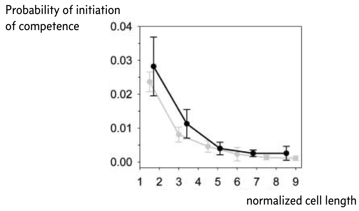
Remember that small copy numbers are a major source of noise. If we could make the copy numbers of the components of the competence circuit have higher copy numbers, we could reduce intrinsic noise. To accomplish this, Süel and coworkers used a ftsW mutant that fails to septate; that is, the cells do not divide. The result is long cells with high copy numbers.
Indeed, when they did this experiment, Süel and coworkers found that cells in their movies were less likely to become competent the longer, and therefore less noisy, the cell was, as shown in the figure below, taken from the 2007 paper. The black curve is from experimental measurements and the gray curve from analysis of stochastic simulations similar to what we show in the next section of this notebook. Here, the y-axis represents the probability that a given cell will become competent before division.
Tunable control of competence
A given cell may go in to competence before it divides. This depends on the amount of time it takes to get kicked into competence by intrinsic noise. Once competent, the cell may remain competent for a short or a long time. This depends on the dynamics as it traverses the competent loop of the phase portrait.
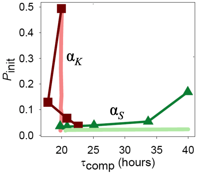
How can these two time scales, that is, the time scale to become competent and the time scale to return from competence, be tuned? Süel and coworkers found that these two time scales can be tuned independently by varying the constitutive expression of comK and comS, respectively, as parametrized by \(\alpha_k\) and \(\alpha_s\).
This stands to reason. If we make more ComK (increase \(\alpha_k\)), this pushes the circuit rightward in the phase portrait, into the competence loop. This results in shorter time to competence.
ComS must be degraded to allows the MecA complex to degrade ComK. So, the faster a cell can get rid of ComS, the faster it can degrade ComK and return from competence. So, if we increase \(\alpha_s\), more ComS is around, and competence is prolonged.
To study this quantitatively, we can take advantage of our ability to sample out of a probability distribution defined by a master equation. With samples, we can compute any quantity we like from them, including the amount of time before the circuit launches into competence and the amount of time it remains in competence. We need to modify some of the Gillespie simulation code to do this. First, we can code up the Gillespie draw, which is the same as in our lecture on the Gillespie SSA.
[20]:
@numba.njit
def gillespie_draw(propensities, population, t, args):
    """
    Draws a reaction and the time it took to do that reaction.
    """
    # Update propensities
    propensity(propensities, population, t, *args)

    # Sum of propensities
    props_sum = np.sum(propensities)

    # Compute time
    time = np.random.exponential(1 / props_sum)

    # Draw reaction given propensities
    rxn = biocircuits.gillespie._sample_discrete(propensities, props_sum)

    return rxn, time
With that in hand, we can code up a function that runs a Gillespie trajectory until competence is initialized (\(k\) goes above a threshold). It records that time, and then continues the trajectory, stopping when competence is exited (\(k\) goes below a threshold).
[21]:
@numba.njit
def competence_times(population_0, args, k_init=10000, k_back=7500, timeout=100000000.0):
    propensities = np.zeros(update.shape[0])
    population = population_0
    k = population[1]

    t = 0
    while t < timeout and k < k_init:
        event, dt = gillespie_draw(propensities, population, t, args)
        population += update[event, :]
        t += dt
        k = population[1]

    # Record time we entered competence
    t_init = t

    while t < timeout and k >= k_back:
        event, dt = gillespie_draw(propensities, population, t, args)
        population += update[event, :]
        t += dt
        k = population[1]

    # Record exit time of competence
    t_exit = t

    return t_init, t_exit
Now we’ll write a function to sample these times repeatedly. For each sample, we will first let the system settle around the stable fixed point in order to get an accurate value for the time to initiate competence. To do this, we will artificially expand the volume of the system using the parameter omega, since we already have seen that this reduces noise. We will then reset omega to its original level and draw the time scales of interest.
[22]:
def sample_competence_time(
    params_ssa,
    settle_time=504000,
    omega_scale=10,
    k_init=10000,
    k_back=7500,
    size=1,
    progress_bar=False,
):
    t_init = np.empty(size)
    t_comp = np.empty(size)

    iterator = tqdm.tqdm(range(size)) if progress_bar else range(size)
    for i in iterator:
        params_ssa_small_omega = params_ssa._replace(
            omega=params_ssa.omega / omega_scale
        )
        population_0 = np.array([10, 100, 10, 400, 500, 0, 0], dtype=int)
        time_points = np.linspace(0, 504000, 3)

        pop = biocircuits.gillespie_ssa(
            propensity,
            update,
            population_0,
            time_points,
            args=tuple(params_ssa_small_omega),
        )

        population_0 = pop[0, -1, :]
        t_init[i], t_exit = competence_times(population_0, tuple(params_ssa))

        t_comp[i] = t_exit - t_init[i]

    return t_init, t_comp
We are now set to do our calculations. We will vary \(\alpha_k\) against the “wild type” \(\alpha_k\) value; that is \(\alpha_k / \alpha_k^{\text{wild type}}\). We will vary the ration \(\alpha_s / \beta_s\). For both, we refer to the conections of the parameters for the discrete model compared to the continuous one. In practice, this means varying \(k_1\) and \(k_4\), respectively, for varying \(\alpha_k\) and \(\alpha_s\).
We will draw 100 samples of these times for each set of parameter values. We will store them in a Pandas DataFrame for convenience. Warning: If you are running this notebook, the following cell takes about 30 minutes to run.
[23]:
alpha_k_ratio = [1, 1.6, 2.5, 4, 6.3, 10]
alpha_s_ratio = [0.0, 0.02, 0.08, 0.15, 0.2, 0.25]
results = {
    "alpha_k_ratio": [],
    "alpha_s_ratio": [],
    "t_init": [],
    "t_comp": [],
}
size = 100

# Run calculations for varying alpha_k with alpha_s = 0
for akr in tqdm.tqdm(alpha_k_ratio):
    params_ssa_new = params_ssa._replace(k1=params_ssa.k1 * akr)
    t_init, t_comp = sample_competence_time(params_ssa_new, size=size)
    results["alpha_k_ratio"] += [akr] * size
    results["alpha_s_ratio"] += [
        params_ssa.k4
        / params_ssa.k5
        * params_ssa.P_comS_const
        / params_ssa.P_comS
    ] * size
    results["t_init"] = np.concatenate((results["t_init"], t_init))
    results["t_comp"] = np.concatenate((results["t_comp"], t_comp))

# Run calculations for varying alpha_s with alpha_k/alpha_k_wt = 1
for asr in tqdm.tqdm(alpha_s_ratio):
    k4 = asr * params_ssa.k5 * params_ssa.P_comS / params_ssa.P_comS_const
    params_ssa_new = params_ssa._replace(k4=k4)
    t_init, t_comp = sample_competence_time(params_ssa_new, size=size)
    results["alpha_k_ratio"] = np.concatenate(
        (results["alpha_k_ratio"], [1] * size)
    )
    results["alpha_s_ratio"] += [asr] * size
    results["t_init"] = np.concatenate((results["t_init"], t_init))
    results["t_comp"] = np.concatenate((results["t_comp"], t_comp))

df = pd.DataFrame(results)
100%|██████████| 6/6 [08:17<00:00, 82.90s/it]
100%|██████████| 6/6 [16:42<00:00, 167.08s/it]
For each of plotting, we can convert the time units from seconds to hours.
[24]:
df['time to competence (hr)'] = df['t_init'] / 3600
df['time competent (hr)'] = df['t_comp'] / 3600
Finally, we will display the plots as ECDFs, a type plot we encountered when discussing copy numbers in cells in our introduction to noise.
[25]:
plot_kwargs = dict(
    frame_height=200,
    frame_width=250,
    x_axis_type="log",
    style="staircase",
    x_range=[1, 2e4],
)

plots = [
    [
        bokeh_catplot.ecdf(
            df.loc[df["alpha_s_ratio"] == 0, :],
            cats="alpha_k_ratio",
            val="time to competence (hr)",
            palette=colorcet.b_linear_blue_5_95_c73[::32],
            x_axis_label=None,
            **plot_kwargs,
        ),
        bokeh_catplot.ecdf(
            df.loc[df["alpha_s_ratio"] == 0, :],
            cats="alpha_k_ratio",
            val="time competent (hr)",
            palette=colorcet.b_linear_blue_5_95_c73[::32],
            x_axis_label=None,
            **plot_kwargs,
        ),
    ],
    [
        bokeh_catplot.ecdf(
            df.loc[df["alpha_k_ratio"] == 1, :],
            cats="alpha_s_ratio",
            val="time to competence (hr)",
            palette=colorcet.b_linear_green_5_95_c69[::32],
            **plot_kwargs,
        ),
        bokeh_catplot.ecdf(
            df.loc[df["alpha_k_ratio"] == 1, :],
            cats="alpha_s_ratio",
            val="time competent (hr)",
            palette=colorcet.b_linear_green_5_95_c69[::32],
            **plot_kwargs,
        ),
    ],
]

# Make legend titles
plots[0][0].legend.title = "αk/αk wt"
plots[1][0].legend.title = "αs/βs"
plots[0][1].legend.title = "αk/αk wt"
plots[1][1].legend.title = "αs/βs"

# Link x-axes
plots[1][0].x_range = plots[0][0].x_range
plots[1][1].x_range = plots[0][1].x_range

bokeh.io.show(bokeh.layouts.gridplot(plots))
The top row has \(\alpha_s\) fixed at zero, and the bottom row has \(\alpha_k/\alpha_k^{\text{wild type}}\) fixed at 1. The left column shows the ECDF of the time to initialize competence and the right columns show the ECDF of the time a cell remains competent. Note that the x-axis scale in all cases is logarithmic.
We will look at the plots one by one.
The upper left plot shows that as constitutive expression of ComK grows (\(\alpha_k\) increasing), the time it takes to initialize competence diminishes. Note, though, that the width of the ECDF grows with increasing time to competence. The coefficient of variation in time to competence grows from about 0.4 to 0.9 over the values of \(\alpha_k\) considered here. (This is calculated in the cell below.)
The upper right plot shows that while the time to initialize competence varies over two orders of magnitude, the amount of time that the cells remain competent is independent of \(\alpha_k\) in this regime.
The bottom right plot shows that increasing \(\alpha_s\) results in greater time in competence. The variation in time in a competent state also grows with increasing \(\alpha_s\), growing from 0.1 to 0.8 in this regime (calculated in a similar was as in the code cell below).
The bottom left plot shows that the time to initialize competence is more or less independent of \(\alpha_s\) in this regime.
Taken together, these results point to independent tuning of the time to initialize competence and the time spend in competence by the strength of constitutive expression of ComK and ComS, respectively. Indeed, Süel and coworkers found this to be the case experimentally. They made Bacillus strains that contains additional copies of comS or comK under control of inducible promoters so that they could artificially adjust \(\alpha_s\) and \(\alpha_k\). They then measured the time to competence and the time spent in competence and found that they could indeed be tuned independently.
[26]:
# Sample calculation of coefficient of variation
df.loc[df["alpha_s_ratio"] == 0, :].groupby("alpha_k_ratio")["t_init"].apply(
    lambda x: x.std() / x.mean()
)
[26]:
alpha_k_ratio
1.0     0.935814
1.6     0.918861
2.5     0.698157
4.0     0.576618
6.3     0.478285
10.0    0.339685
Name: t_init, dtype: float64
Computing environment
[27]:
%load_ext watermark
%watermark -v -p numpy,scipy,numba,bokeh,bokeh_catplot,colorcet,tqdm,biocircuits,jupyterlab
CPython 3.7.7
IPython 7.13.0

numpy 1.18.1
scipy 1.4.1
numba 0.49.0
bokeh 2.0.2
bokeh_catplot 0.1.8
colorcet 2.0.2
tqdm 4.45.0
biocircuits 0.0.16
jupyterlab 1.2.6