Homework 6.1: A possible mechanism for bursty gene expression (100 pts)

---

Lengyel and Morelli (PRE, 2017) considered a model for regulation of gene expression that may lead to bursty expression. The authors noted that many genes occurring in organisms from bacteria to humans are autorepressed, and furthermore that clusters of binding sites for the same transcription factor also commonly occur. They then proposed a simple model for the production of an autorepressed gene, shown below.

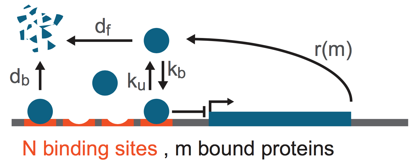
The protein gene product is made with a rate \(r(m)\), where \(m\) is the number of proteins bound to the \(N\) identical binding sites near the promoter. The binding is reversible with binding and unbinding rates respectively being \(k_b\) and \(k_u\). Finally, the bound proteins decay with rate \(d_b\) and free proteins decay with rate \(d_f\). To complete the notation, we define the number of unbound proteins in a cell as \(n\).

In this problem, you will use Gillespie simulations (SSAs) to arrive at some of the key results of the Lengyel and Morelli paper.

a) Lengyel and Morelli wrote a master equation to describe the dynamics as

\begin{align} \frac{\mathrm{d}P(n,m,t)}{\mathrm{d}t} = &\; r(m)\left(P(n-1,m,t) - P(n,m,t)\right) \nonumber \\[1em] &+ k_b\left[(N-(m-1))(n+1)P(n+1, m-1, t) - (N-m)nP(n,m,t)\right] \nonumber \\[1em] &+ k_u\left[(m+1)P(n-1,m+1,t) - mP(n,m,t)\right] \nonumber \\[1em] &+ d_f\left[(n+1)P(n+1, m,t) - n(P(n,m,t))\right] \nonumber \\[1em] &+d_b\left[(m+1)P(n,m+1,t) - mP(n,m,t)\right]. \end{align}

By defining \(\gamma \equiv d_b/d_f\), and appropriately redefining the other parameters, we can eliminate a parameter and write the master equation as

\begin{align} \frac{\mathrm{d}P(n,m,t)}{\mathrm{d}t} = & r(m)\left(P(n-1,m,t) - P(n,m,t)\right) \nonumber \\[1em] &+ k_b\left[(N-(m-1))(n+1)P(n+1, m-1, t) - (N-m)nP(n,m,t)\right] \nonumber \\[1em] &+ k_u\left[(m+1)P(n-1,m+1,t) - mP(n,m,t)\right] \nonumber \\[1em] &+ (n+1)P(n+1, m,t) - n(P(n,m,t)) \nonumber \\[1em] &+\gamma\left[(m+1)P(n,m+1,t) - mP(n,m,t)\right]. \end{align}

Given this master equation, write down the transitions and their propensities that you will use to define a Gillespie simulation.

b) For our simulations, we will take

\begin{align} r(m) = \left\{\begin{array}{lcl} r_0 && \text{if } 0 \le m \le M,\\ 0 && \text{otherwise}. \end{array} \right. \end{align}

This means that the repression is very sharp. This leaves us with six parameters we need to define, \(r_0\), \(k_b\), \(k_u\), \(\gamma\), \(N\), and \(M\). For all of our simulations, we will take \(k_b = k_u = 335.5\). We will also take \(\gamma = 1\) (except for part (f), see below). We will consider various values of \(N\) and \(M\). That is, we will look at how the number of binding sites and the threshold for repression affect bursty expression and noise. With these parameters set, the value of \(r_0\) is set such that the long-time average total number of proteins, \(n_t = m + n\), is (approximately) 20. We do this so that we can make clear comparisons between parameter sets; we want them all to have the same average expression level and we can then explore bursty dynamics and noise. Finding the values of \(r_0\) to enforce that the long-time averages are all about 20 is nontrivial, and we have done that for you. You can download relevant parameter sets here.

It will help you to easily access these parameters using the Python package Pandas. The code below shows how to load in the parameters and select the set you would want for \(N = 5\), \(M = 0\), and \(\gamma = 1\).

import pandas as pd

# Load in the parameters into a Pandas DataFrame
df = pd.read_csv("autorepression_params.csv")

# Get index of parameter set we want
ind = df[(df.N == 5) & (df.M == 0) & (df.gamma == 1.0)].index[0]

# Extract the row out of the DataFrame
r = df.loc[ind, :]

# Specify parameters
r0 = r["r0"]
kb = r["kb"]
ku = r["ku"]
gamma = r["gamma"]
N = r["N"]
M = r["M"]

You would use similar syntax for any other entry of interest, e.g., for the parameter set with \(N=14\), \(M=9\), and \(\gamma = 0\):

ind = df[(df["N"] == 14) & (df["M"] == 9) & (df["gamma"] == 0.0)].index[0]

Now that you know how to access parameters, you can code up and run a simulation. For your first simulation, use the parameter set \(N = 5\), \(M = 0\), and \(\gamma = 1\). Since \(M = 0\), expression is shut down if any proteins are bound to any of the binding sites. Perform a Gillespie simulation starting with \(n = m = 0\) going from time \(t = 0\) to \(t = 30\). Compute the total number of protein products (\(n_t = m + n\)) over time. Plot the result. Do you see bursts?

c) I suspect you said you saw bursts in part (c). (If you didn’t, you should probably try troubleshooting your code.) Re-run the simulation much longer this time; up to about \(t = 500\) will do. Using this trajectory, compute the burst size (number of proteins made per burst) and the inter-burst times.

Recall that in class, we showed from the Cai, Friedman, and Xie paper that the burst size for expression of β-gal in yeast was geometrically distributed. We assumed that the inter-burst times were exponentially distributed, which gives that the number of proteins is negative binomially distributed. Based on the burst sizes and inter-burst times you computed, do you think they are respectively geometrically and exponentially distributed in this model?

d) In class, we will discuss a paper by Singer, et al., in which they use mRNA FISH to show that the number of RNA transcripts in a population of cells are negative binomially distributed. Now you can simulate that experiment. Perform 200 Gillespie simulations up to time \(t = 20\). You now have samples of the number of proteins, \(n_t\), in 200 “cells” at time \(t = 20\). Do these values appear to be negative binomially distributed?

e) It is often thought that negative autorepression can reduce noise. Here, we will quantify noise, as we did in lecture by the coefficient of variation,

\begin{align} \eta = \frac{\sqrt{\left\langle n_t^2\right\rangle - \left\langle n_t\right\rangle^2}}{\left\langle n_t\right\rangle}. \end{align}

• 1. Compute the coefficient of variation for \(N \in [1, 14]\) for \(M = 0\) and \(\gamma = 1\). Describe your strategy for how you compute the coefficient of variation. Make a plot of \(\eta\) versus \(N\) and comment on what you see. Does increasing the number of binding sites reduce noise?

• 2. We will now look at how the threshold number of bound sites before repression affects now. Say we have \(N = 14\) binding sites, again with \(\gamma = 1\). Compute \(\eta\) for \(M \in [0, 14]\) and plot the result. Are there values for \(M\) for which the noise is lower than the single binding site (\(N=1\)) case?

f) (not graded) If you like, for fun, investigate what happens if the bound proteins cannot degrade (\(\gamma = 0\)).