Homework 8.1: Controlling p53 levels (70 pts)

---

import numpy as np

---

p53 is an important protein for tumor suppression, DNA damage repair, cell cycle regulation, and more. In their 2012 paper, the researchers in Galit Lahav’s group investigated how temporal dynamics of p53 controls cell fate in MCF-7 cells, a breast cancer cell line. It had been previously observed that p53 levels oscillate upon exposure to stress due to γ radiation. To instead study how cells respond to sustained levels of p53, the authors controlled p53 levels using the drug Nutlin-3. To do this, they devised a program for adjusting Nutlin-3 levels in the cell culture that would keep the p53 levels at a constant high level. They based this program on a mathematical model of the p53 circuit (shown in the figure below) that they developed and parametrized in an earlier paper.

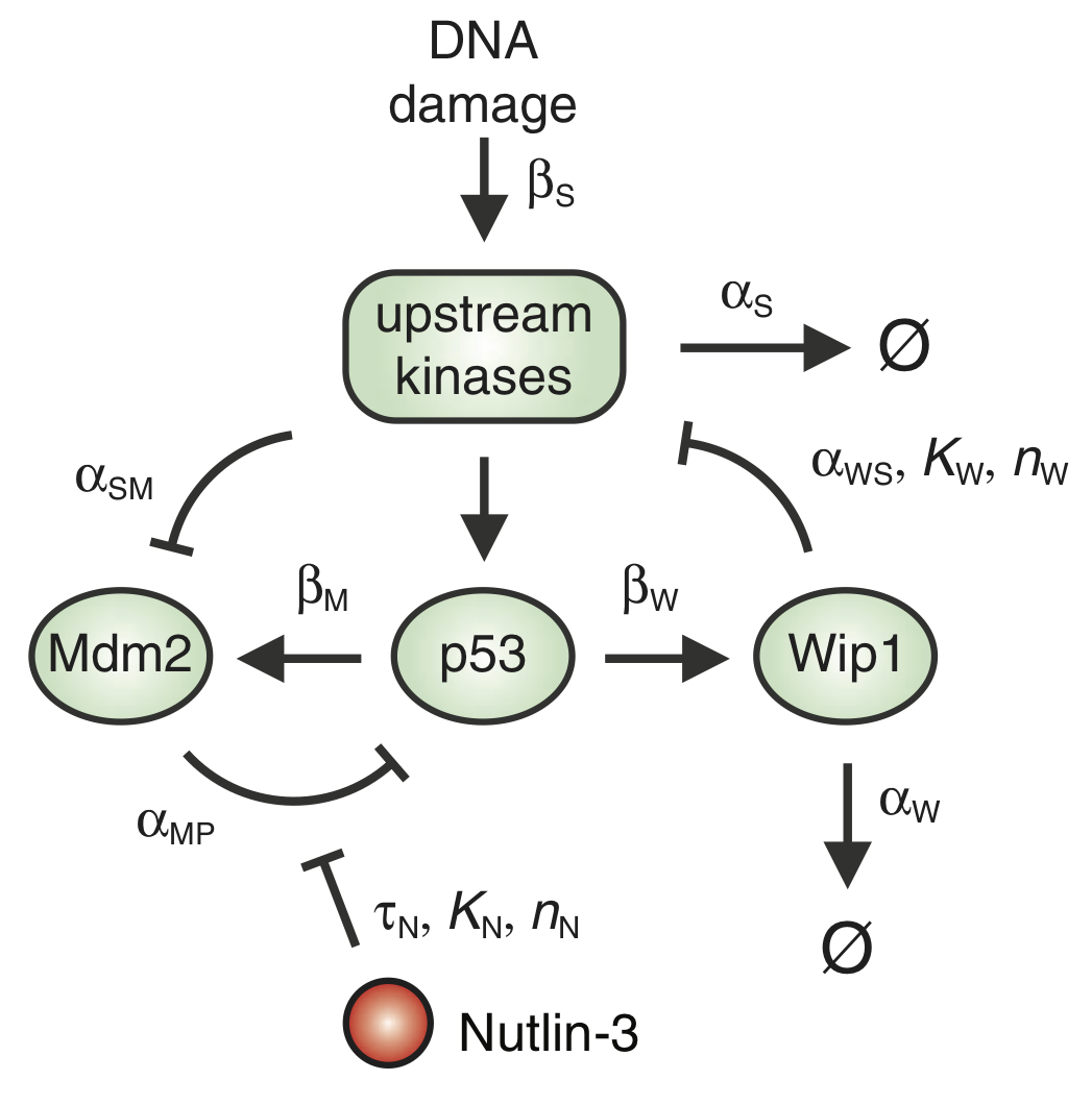
The p53 levels oscillate due to a delays in the autoinhibitory loops mediated by Mdm2 and Wip1. The dynamical equations for this circuit, as presented in the paper, are

\begin{align} \frac{\mathrm{d}P_i}{\mathrm{d}t} &= \beta_\mathrm{P} - \frac{\alpha_\mathrm{MP_i} \, M\,P_i}{1+\left(N(t-\tau_\mathrm{N})/K\right)^{n_\mathrm{N}}} - \beta_\mathrm{SP}\,P_i\,\frac{(S/T_\mathrm{S})^{n_\mathrm{S}}}{1 + (S/T_\mathrm{S})^{n_\mathrm{S}}} - \alpha_\mathrm{P_i}\, P_i,\\[1em] \frac{\mathrm{d}P_a}{\mathrm{d}t} &= \beta_\mathrm{SP}\,P_i\,\frac{(S/T_\mathrm{S})^{n_\mathrm{S}}}{1 + (S/T_\mathrm{S})^{n_\mathrm{S}}} - \frac{\alpha_\mathrm{MP_a} \, M\,P_a}{1+\left(N(t-\tau_\mathrm{N})/K\right)^{n_\mathrm{N}}},\\[1em] \frac{\mathrm{d}M}{\mathrm{d}t} &= \beta_\mathrm{M}\,P_a(t-\tau_\mathrm{M}) + \beta_{M_i} - \alpha_\mathrm{SM}\,S\,M - \alpha_M\,M,\\[1em] \frac{\mathrm{d}W}{\mathrm{d}t} &= \beta_\mathrm{W}\,P_a(t-\tau_\mathrm{W}) - \alpha_\mathrm{W}\,W,\\[1em] \frac{\mathrm{d}S}{\mathrm{d}t} &= \beta_\mathrm{S}\,\theta(t) - \alpha_\mathrm{WS}\,S\,\frac{(W/T_\mathrm{W})^{n_\mathrm{W}}}{1 + (W/T_\mathrm{W})^{n_\mathrm{W}}} - \alpha_\mathrm{S}\,S. \end{align}

Here, \(P_i\) and \(P_a\) denote the concentrations of inactive and active p53, respectively. \(M\) and \(W\) are respectively the concentrations of Mdm2 and Wip1. The concentration of the DNA damage signal is denoted as \(S\). Finally, \(N\) is the externally imposed concentration of Nutlin-3. The function \(\theta(t)\) is the Heaviside function,

\begin{align} \theta(t) = \left\{\begin{array}[ll] 00 & t < 0 \\ 1 & t \ge 0. \end{array} \right. \end{align}

The parameters for the model are given in the code cell below. Before proceeding, take a moment and make sure you understand the physical meaning of each term in the equations.

# Parameters for p53 model
alpha_MPi = 5
alpha_Pi = 2
alpha_MPa = 1.4
alpha_SM = 0.5
alpha_M = 1
alpha_W = 0.7
alpha_WS = 50
alpha_S = 7.5
beta_P = 0.9
beta_SP = 10
beta_M = 0.9
beta_Mi = 0.2
beta_W = 0.25
beta_S = 10
tau_N = 0.4     # hours
tau_M = 0.7     # hours
tau_W = 1.25    # hours
K = 2.3         # µM
n_N = 3.3
n_S = 4
n_W = 4
T_W = 0.2
T_S = 1

a) Solve the equations numerically with \(N = 0\). Plot the solution along with the experimental measurements from the Purvis, et al. paper, given in the Numpy arrays below. This helps verify that the model gives results similar to what you would observe experimentally.

# Time points (in units of hours)
time = np.array([0, 1, 2, 3, 4, 5, 6, 7, 8, 12])
relative_total_p53_conc = np.array(
    [0.13, 0.69, 1.00, 0.87, 0.60, 0.35, 0.34, 0.54, 0.61, 0.42]
)

b) Come up with a program for controlling the Nutlin-3 concentration so as to bring the total p53 level to a sustained value similar to that of its maximum value during oscillations in the absence of Nutlin-3. I.e., choose a function \(N(t)\) to give a sustained level of p53 that is approximately unity (in the units specified by the parameter values). You might want to consider experimental constraints; for example that you might want to have only a few steps where the Nutlin-3 concentrations are adjusted to ease experimentation. Show a plot verifying that your scheme works.