Homework 8.2: Turing patterns with expanders (70 pts)
8.2: Turing patterns with expanders (70 pts)
In this problem, we will explore scaling of Turing patterns, described by Werner, et al. (PRL, 2015).
As discussed in lecture, Turing patterns tend to have a wavelength that is independent of the size of the system, which means that they do not scale. Werner and coworkers propose a model for interactions of an expander (E) with the classical Turing activator (A)-inhibitor (B) components. The model is shown below.
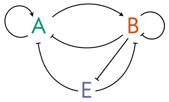
The color coding of the species will be useful to use in your plots. The hex codes are ['#1b9e77', '#d95f02', '#7570b3'], respectively, for A, B, and E.
In this problem, we will consider only a one-dimensional system such that \(\nabla^2 = \partial^2/\partial x^2\).
a) We will consider the expander in the next part of the problem. For now, consider only the activator-inhibitor circuit.
\begin{align} \frac{\partial a}{\partial t} &= D_A\,\frac{\partial^2 a}{\partial x^2} + \beta_A\,\frac{(a/k_a)^n}{(a/k_a)^n + (b/k_b)^n} - \gamma_A a \\[1em] \frac{\partial b}{\partial t} &= D_B\,\frac{\partial^2 b}{\partial x^2} + \beta_B\,\frac{(a/k_a)^n}{(a/k_a)^n + (b/k_b)^n} - \gamma_B b. \end{align}
Explain each term in the following set of PDEs and highlight any assumptions (most of which were made for simplicity) that were made in the modeling. Do these PDEs make sense for this circuit?
Show that we can nondimensionalize this PDEs to be
\begin{align} \frac{\partial a}{\partial t} &= d_a\,\frac{\partial^2 a}{\partial x^2} + \beta_a\,\frac{a^n}{a^n + b^n} - \gamma_a\,a \\[1em] \frac{\partial b}{\partial t} &= \frac{\partial^2 b}{\partial x^2} + \beta_b\,\frac{a^n}{a^n + b^n} - b, \end{align}
where \(a\), \(b\), \(x\), and \(t\) are now dimensionless.
Consider now just the chemical part of the above system; that is, neglect diffusion. Write down an expression for the steady state concentrations of A and B. Since we neglected diffusion, this is the homogeneous steady state.
Starting from a small perturbation of the nonzero homogeneous steady state, numerically solve the coupled PDEs. Use no-flux boundary conditions. Plot the resulting steady state concentration profiles for \(a\) and \(b\). Do this using the following parameters: \(d_a = 0.033\), \(\beta_a = 2.5\), \(\beta_b = 10\), \(\gamma_a = 0.5\), and \(n = 5\). Do this five times, once each for the total dimensionless length of the system being 5, 10, 20, 40, and 80. Comment on the pertinence of these results with respect to scaling.
b) We will now consider the system in the presence of an expander, E. The expander functions as a degron; it regulates degradation of the activator and inhibitor. Similarly, the inhibitor B acts as a degron for the expander E. The new dimensional equations are
\begin{align} \frac{\partial a}{\partial t} &= D_A\,\frac{\partial^2 a}{\partial x^2} + \beta_A\,\frac{(a/k_a)^n}{ (a/k_a)^n + (b/k_b)^n} - \kappa_A\, e a\\[1em] \frac{\partial b}{\partial t} &= D_B\,\frac{\partial^2 b}{\partial x^2} + \beta_B\,\frac{ (a/k_a)^n}{ (a/k_a)^n + (b/k_b)^n} - \kappa_B\,e b,\\[1em] \frac{\partial e}{\partial t} &= D_E\,\frac{\partial^2 e}{\partial x^2} + \beta_E - \kappa_E\,e b. \end{align}
Show that these equations may be nondimensionalized to read
\begin{align} \frac{\partial a}{\partial t} &= d_a\,\frac{\partial^2 a}{\partial x^2} + \beta_a\,\frac{ a^n}{ a^n + b^n} - \kappa_a\,e a \\[1em] \frac{\partial b}{\partial t} &= \frac{\partial^2 b}{\partial x^2} + \beta_b\,\frac{ a^n}{ a^n + b^n} - e b,\\[1em] \frac{\partial e}{\partial t} &= d_e\,\frac{\partial^2 e}{\partial x^2} + 1 - \kappa_e e b. \end{align}
Note that the length by which you nondimensionalize space (\(x\)) and the time scale by which you nontimensionalize time (\(t\)) will be different than in part (a).
There are no homogeneous steady states for this system. For our initial “steady state” when doing the numerical calculations, we will take \(e_0 = 1\) and solve for the values of \(a\) and \(b\) such that \(\mathrm{d}a/\mathrm{d}t = \mathrm{d}b/\mathrm{d}t = 0\). Nevermind that for this “steady state,” \(\mathrm{d}e/\mathrm{d}t \ne 0\). Again, starting from a small perturbation of this “steady state,” numerically solve the coupled PDEs using no-flux boundary conditions. Plot the resulting steady state concentration profiles for \(a\) and \(b\). Do this using the same parameters as in part (a-4), with additional parameters \(d_e = 0.33\), \(\kappa_a = 0.5\), and \(\kappa_e = 1\). Again, do this five times, once each for the total dimensionless length of the system being 5, 10, 20, 40, and 80. (You can do it for more lengths if you like.) Comment on the pertinence of these results with respect to scaling.
c) Comment qualitatively on how the expander works to scale the Turing patterns. By what other means (other than mutual inhibition of B and inhibition of A) might an expander operate? Remember, these models are postulates of what might be happening in developing organisms, so it is useful to dream up alternatives.